Data analysis and statistical approaches
Contents
General description
These methods are generally data analysis methods where the general aim is to find a small number of shape functions or sinusoidal functions, or a small number of eigenvectors, that resolve with sufficient accuracy the spatial and temporal properties of the data. This data may relate to some of the forcings, like the waves, winds and currents, or to the bathymetry. An approximation of the data to about 80% to 85% may be sufficient for some applications and in such cases maybe 2 to 5 functions or eigenvectors may be chosen. However, it is generally preferably to be able to approximate the original data set with at least 90% (Gilmore and Lefranc, 2003)[1], especially when the objective is to find a set of variables embed the original dataset, as is the case for some chaotic techniques (described in more detailed below). Nonetheless, in coastal engineering it is common practice to approximate the data of interest with up to 5 functions or eigenvectors (see for example Rattan et al. 2005[2]or Li et al., 2005[3]), in order to simplify the analysis. Such methods are described in more detail below, following the reviews by Southgate et al. (2003) [4] and Larson et al. (2003)[5]. Bulk statistics methods, discussed by Larson et al. (2003), are briefly summarized below. Then follows an analysis methods for beach level data. Finally some advanced linear and nonlinear data analysis methods are presented.
Bulk statistics methods
This method uses the statistical properties of a data time series (mean, range, variance, correlation, etc) to characterise the behaviour of a system. As such, the implementation of the method is very simple, and it has thus been extensively used in many fields, including coastal research. These methods have traditionally been applied to short-term and long-term wave statistics, for instance. In short-term wave analysis, a wave height may be analysed directly, or after being decomposed in a sum of sinusoidal functions (that is, using a Fourier expansion), from which the moments of the data may be extracted. These methods allow, also, to calculate the properties of extreme events according to their probability of occurrence, and are thus very useful in coastal structure design (Larson et al., 2003). In relation to morphodynamics, statistical properties of the temporal and spatial evolution of different coastal features have been investigated, in particular as a preliminary step in studies when Principal Component Analyses are involved (see section 3.3).
Linear analysis of beach level data
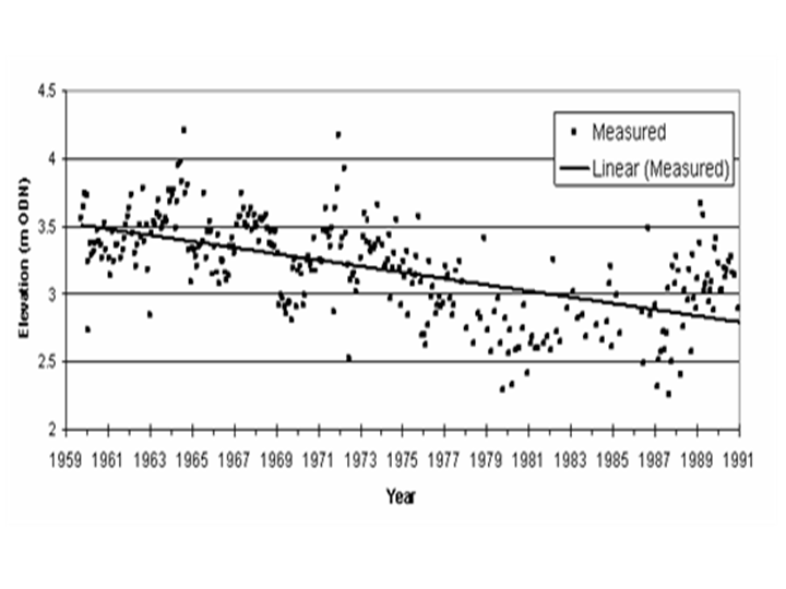
The linear analysis of beach level data is demonstrated here using a set of beach profile measurements carried out at locations along the Lincolnshire coast (UK) by the National Rivers Authority (now the Environment Agency[link]) and its predecessors between 1959 and 1991, as described in HR Wallingford (2006c). Locations backed by a seawall were chosen and a time series of beach levels at a set point in front of the seawall at Mablethorpe Convalescent Home are shown in Figure 1.
Use of trend line for prediction
Straight lines fitted to beach level time series give an indication of the rate of change of elevation and hence of erosion or accretion. The measured rates of change are often used to predict future beach levels by assuming that the best-fit rate from one period will be continued into the future. Alternatively, long-term shoreline change rates can be determined using linear regression on cross-shore position versus time data.
Genz et al. (2007)[6] reviewed methods of fitting trend lines, including using end point rates, the average of rates, ordinary least squares (including variations such as jackknifing, re-weighted least squares, weighted least squares and weighted re-weighted least squares) least absolute deviation (with and without weighting functions). Genz et al. recommended that weighted methods should be used in uncertainties are understood, but not otherwise. The ordinary least squares, re-weighted least squares, jackknifing and least absolute deviation methods were preferred (with weighting, if appropriate). If the uncertainties are unknown or not quantified then the least absolute deviation methods is preferred.
The following question then arises: how useful is a best-fit linear trend as a predictor of future beach levels? In order to examine this, the thirty years of Lincolnshire data have been divided into sections: from 1960 to 1970, from 1970 to 1980, from 1980 to 1990 and from 1960 to 1990, for most of the stations. In each case a least-squares best-fit straight line has been fitted to the data and the rates of change in elevation from the different periods are shown below:
- From 1960 to 1970 the rate of change was -17mm/year;
- From 1970 to 1980 the rate of change was -63mm/year;
- From 1980 to 1990 the rate of change was +47mm/year.
- From 1960 to 1990 the rate of change was -25mm/year.
The data above indicates that 10-year averages provide little predictive capability for estimating the change in elevation for the next 10-years, let alone for the planning horizon that might need to be considered for a coastal engineering scheme. Few of the 10-year averages are close to the 30-year average.
A prediction horizon is defined as the average length of time over which a prediction (here an extrapolated trend) produces a better level of prediction of future beach levels than a simple baseline prediction. Sutherland et al. (2007)[7] devised a method of determining the prediction horizon for an extrapolated trend using the Brier Skill Score (Sutherland et al., 2004[8]). Here the baseline prediction was that future beach levels would be the same as the average of the measured levels used to define the trend. A 10 year trend was found to have a prediction horizon of 4 years at Mablethorpe Convalescent Home (Figure 2). Similar values have been found at other sites in Lincolnshire.
Gaussian distribution of residuals
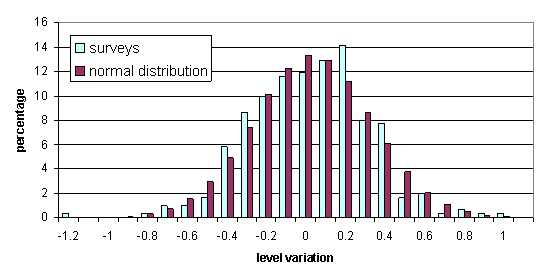
The good news is that distribution of residual (i.e. de-trended) beach levels seems to follow the common assumption that it is Gaussian, or normal distribution, as shown for the Mablethorpe data in Figure 2.
Linear and nonlinear analysis of datasets
Wavelets
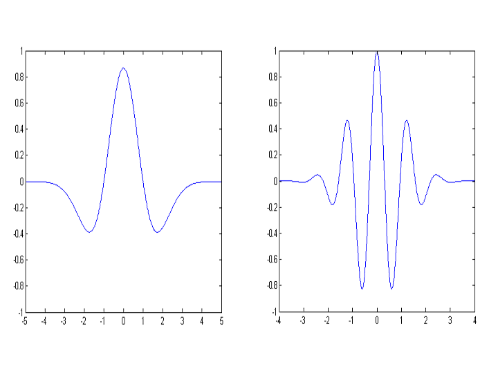
The wavelet technique is similar to a Fourier analysis approach, where the signal is approximated by some basis functions, which in wavelet analysis are simply wavelet functions. The advantage of wavelets over Fourier based methods is that wavelets are localized both in frequency and time, where as sinusoidal functions are only localized in frequency (Burrus et al., 1998[9]). Time resolution is achieved with wavelets by using a scalable modulated window that is shifted along the signal (C. Valens, http://perso.orange.fr/polyvalens/clemens/wavelets/wavelets.html#eq1, accessed 12/03/07). Other important properties of wavelets are that their mean is zero and their average squared norm is unity. Also, generally a very small number of wavelets is needed to reconstruct a function with sufficient accuracy. A very well known example of a wavelet is the Mexican hat, shown in Figure 3 on the left, which has only one peak. Figure 3 on the right shows the Morlet wavelet, with 5 peaks. These examples are examples of mother wavelets, which may be dilated and transformed to form the basis. The first wavelet function was developed by Haar (1910).[10] Wavelets have traditionally been used in data analysis to increase the signal-to-noise ratio, and also to compress the data to only a few wavelet functions.
Wavelets were first used in coastal morphodynamics by Sarah Little et al. (1993) [11] to analyse large scale (of the order of 100 to 1000 kms) bathymetric evolution offshore the Hawaian islands; the wavelets the authors adopted for this analysis were Daubechies wavelets, a family of discrete orthogonal wavelets introduced by I. Daubechies (1988).[12] Thanks to the wavelet scale analysis and application of a wavelet transform, the authors were able to discover a small, low-frequency topographic feature of around 200 kms in length, whose details suggest it is a slow-spreading rift. After this pioneering work, other topography identification investigations have followed (eg. Little et al., 1996). More recently, Li et al. (2005) analysed nearshore beach profile variability in Duck, North Carolina (USA); the space scales in this case were, instead, of the order of 0.1 kms. The objective of the study was to analyse both time and space variability of the bathymetry. Thus, the authors chose Daubechies’ wavelets as a base and adopt an adapted maximum overlap discrete wavelet transform (AMODWT), as both are very suitable for decomposition of signals with strong space and time variations.
Li et al. (2005) study in detail a bathymetry profile that has been thoroughly surveyed since 1981. They identify the variance across the profile as nonstationary, with largest variations in the sandbank region; this region occurs between 100 and 400-500 m offshore. Within this region, the 128-256 m spatial scale contains most of the information, and makes the largest contribution to the variance for all the months surveyed. The authors suggest this is because high-energy waves would affect the bathymetry from the surf zone to deep water, that is for distances of the order of 100 meters. However, why high-energy waves, rather than the more ubiquitous moderate wave conditions, should have a larger effect on the wavelet decomposition is unclear. It is worth noting that the largest variations of the 128m occur in the sandbar region, indicating this is the region where the morphology evolves the most, which is to be expected. Contrary to the spatial scales, the temporal wavelets contribute differently to the total variance depending on the month considered and the position along the profile. However, it may be pointed out that the two temporal wavelets that span from 32-64 and 64-128 months, respectively, contain most of the variance. Contributions of lower order appear as large peaks in the profiles, indicating they are mostly event-related, rather than part of the average trend. This is highlighted by the authors with several examples. This work proves wavelets are a useful technique in signal decomposition and have great potential in coastal research.
Empirical Orthogonal Functions (EOF) and Singular Spectrum Analysis (SSA)
The objective of the EOF and SSA techniques is for the variance of the original data set to be resolved with good accuracy with only a few shape functions. This is achieved by choosing the EOF or SSA modes in such a way that the variance resolved by each mode decreases with mode number. In this way, most of the variance of the original data set is resolved by the first few modes. A morphological variable sampled in space and time may be decomposed into a set of modes that resolve the spatial features and an another set of temporal modes, each composed a number of orthonormal eigenvectors (that is, these vectors are orthogonal and have norm 1). To each product of two eigenvectors (of which one is spatial and another one is temporal) corresponds an eigenvalue, that is, a constant, which is a measure of the variance resolved by that eigenvector product ; as explained above, the order of the eigenvectors is chosen so that the variance resolved decreases monotonically as the modes of the eigenvectors increase. These methods (both EOF and SSA, or more generally Principal Component Analysis - PCA - techniques) involve thus solving an eigenvalue problem for the covariance matrix based on the data, where this matrix may have the space sampling in its columns and the temporal sampling in its rows (Preisendorfer, 1988, as cited by Larson, 2003). The EOF methods has been used with success to analyse nearshore beach topography, as will be described below. However, the technique may not be appropriate for studies of bar dynamics as eigenfunctions are fixed in space but bars, on the contrary, are wave-like patterns that travel in time. Extended EOFs and Complex Principal Component Analysis, both modifications of EOFs, do not have such shortcoming; however, they rely on time-lagged data, and thus the data needs to be sampled at constant time intervals. This is not usual in coastal applications, as noted by Larson et al. (2003), but may be achieved via data interpolation. It is of interest to note that the SSA technique, described in more detail further below, is used generally for chaotic characterization studies. We first discuss, in the paragraph below, some applications of EOFs. Larson et al. (2003) cite three papers (Hayden et al. 1975 [13], Winant et al., 1975 [14] and Aubrey et al., 1979[15]) as pioneering applications of EOFs in coastal morphology, in particular for beach profile behaviour; these researchers, as Larson et al. (2003) point out, observed the lower order EOF modes could be related to particular coastal features, i.e. the mean profile, bars and berms, and low-tide terraces to the first, second and third order modes, respectively. Therefore, these studies also constitute first attempts of coastal characterization via EOFs. More recently, the EOF method together with a moving window model were used by Wijnberg and Terwindt (1995) [16] to divide the Dutch coast into regions according to their characteristic patterns of behaviour. They analysed 115 kms of Dutch coast via 14 thousand near cross-shore transects at generally 250 m longshore intervals. These regions vary form 5 to 42 kms in size, each characterised mainly by what the authors define as ‘secondary’ features, that is features diverging from the mean profile such as mounds or sandbars (this example and those mentioned below are such that the mean has not been removed from the data). The authors observed subdecadal shifts of shoreline positions and speculate this could be related to sandbar dynamics. Larson et al. (2003) applied the same technique of Wijnberg and Terwindt (1995) to nearshore topography in a Dutch and a German coastal area. For the Dutch coastal site, the modes were related to the coastal features, with similar results as in Aubrey (1979) except that third EOF was shifter 90 degrees in phase with respect to the second and was also related to the bar system. For the german site, the technique was applied to study beach nourishment effects on topography evolution at a beach resort that has suffered from severe erosion in the past (Dette and Newe, 1997).[17] In this case the first EOF indicated an increase in mean elevation. Similarly to other EOF analysis at other sites infilled sites, rapid changes occur at the beginning and were then followed by gradual adjustment to an equilibrium. In general the process takes one year if fill is nearshore, or considerably longer if the fill is at the berm, as Larson et al. (2003) observed. A particular modification of the EOFs, namely Singular spectrum analysis (SSA), has been used to identify chaotic properties of a system, that is, to determine the number (embedding dimension) of independent variables that are needed to describe the system, and the properties of the attractors in such system. SSA was extensively discussed by Southgate et al. (2003), and the main points raised by the authors are summarized here. Firstly, in the case of SSA the data matrix has in its columns not all the measured time series at all times, but the data at successive equitemporal lags, up to the maximum shift needed for a full system’s description. The number of columns of the data matrix defined as such is called the embedding dimension, d, and the SSA will not resolve periods longer than that corresponding to d. SSA may be used not only chaotic characterization, but also for noise reduction, data detrending, oscillatory characterization, or forecasting. Example applications to coastal morphology, given by Southgate et al. (2003), relate to long-term shoreline evolution. However, in general this technique has not been applied to coastal research, but rather to climatology (e.g. Ghil et al., 2002 [18]).
Principal Oscillation Patterns and PIP
In a Principal Oscillation Pattern (POP) analysis the data is analysed using patterns based on approximate forms of dynamical equations so may be used to identify changing patterns, such as standing waves and migrating waves (Larson et al, 2003). POP is a linearised form of the more general Principal Interaction Pattern (PIP) analysis. A POP analysis using the long-term Dutch JARKUS dataset of cross-shore beach profiles (Jansen, 1997[19]) showed that POP systematically lost 4% to 8% more data than an EOF analysis. The prediction method was optimised using 8 POPs as adding more POPS included more of the noise. Różyński and Jansen (2002)[20] applied POP analysis to 4 beach profiles at Lubiatowo (Poland) and recommended that an EOF analysis be carried out first.
Neural Networks
Background
Hodgkin and Huxley (1952)[21] performed pioneering experimental studies on current propagation along the giant axon of a squid, consequently developing the first detailed mathematical model of neuron dynamics. The model is the first to include multiple ion channels and synaptic processes, as well as realistic neural geometry, (Gerstner and Kistler, 2002)[22]. Following this work, several researchers started to study neurons as an interconnected system, developing the theory of Neural Networks. The term “perceptron” was introduced by Rosenblatt (1961)[23] during this time to refer to an artificial neuron, rather than a natural one. However, according to Kingston (2003) [24], the origin of artificial neurons may be traced back to McCulloch and Pitts (1943). [25]
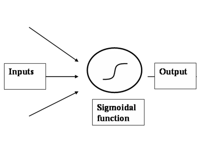
In Neural Networks, the propagation of the current along the main body of the cell and subsequent release of ions in the synapses constitutes a feedforward (or feedbackward) mechanism between perceptrons. This property has been extensively exploited in artificial Neural Network modeling. The release of ions and then retrieval at the synaptic end of the connected perceptron may be modeled as a sigmoidal function, as that shown inside the ellipse in Figure 4 below. This sigmoidal function represents an excitation threshold density for the neuron population, that is an average population activity (other models have used a step function or a linear function to simulate the excitation threshold between perceptrons, but such representations have limited applicability). The number of inputs and the form of the transformation function may vary, and the precise form of the output may vary accordingly. Sigmoidal functions are important because they are nonlinear and continuous, but many other options are possible. Also, different inputs may be transformed using different functions, and may be transformed as well several times. The type of function, the number of functions used in each layer (or each transformation step), and the number of layers may be modified so that the perceptron may reproduce certain characteristics of the phenomenon under study. This can be to be able to reproduce a certain behavior of a group of cells, or simply to reproduce characteristics of some data that is being analysed using a perceptron, regardless of the particular application.
Although Artificial Neural Networks models were originally developed to understand dynamics of brain cells, many applications exist now where artificial neural networks are used for analysis of data. Also, once the Neural Network parameters have been calibrated using the input variables, the model can then be used as a predictive tool. This is how Artificial Neural Networks have been applied to coastal morphodynamics.
Applications to coastal morphodynamics
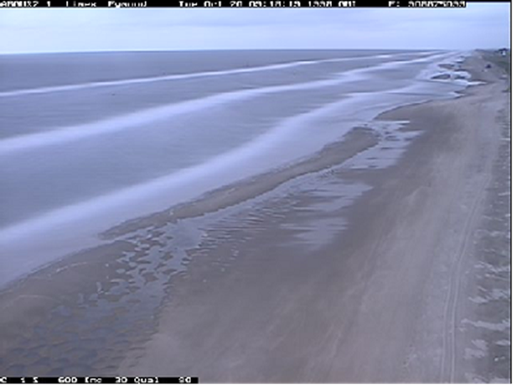
Several applications to coastal morphodynamics using Neural Networks have been developed in the past. Here we will mention several examples described in Kinston, as well as a particular Neural Network model applied to the analysis of sandbank evolution. For the purposes of coastal modeling several input data may be considerer. Of significance one may consider tidal measurements, shoreline evolution, bathymetry evolution, wave height, period and direction, to name but a few. Then the modeler needs to select the appropriate Network parameters that reproduce most closely the observations. If the model needs many different layers, or different functions are each layer, then the processing power of the model is weak, but if the model is efficient with a small number of parameters then the processing power increases. It is also important to assess which input variables are the most relevant. Many applications relate to wave and tidal forecasting (Deo and Sridar Naidu, 1999[27]and Tsai and Lee, 1999 [28]). Concerning the sea floor evolution, several studies have concentrated on sandbank evolution, for instance to predict location and motion of sandbanks from video images. Figure 5 is an example of video imaging at Egmond aan Zee, The Netherlands. A Neural Network technique is used to correct the quality of the image. Another application of Neural Networks concerns the dynamics of the sandbanks, that is, how they evolve with time. An example of this type of application is in Rattan, Ruessink and Hsieh (2005). Rattan et al.[29] used three different data analysis methods to study the behaviour of three sandbank systems, one in Egmoond aan Zee, A system in Hasaki, Japan, and the sandbank behaviour in Duck Site, North Carolina. The three methods were based on Principal Component Analysis, but the most complex method included a Neural Network technique. The properties of the each system were characterized according to how ell each of the methods reproduced the observed behavior. If, say, a simple linear model produced the results with the same accuracy as a nonlinear method, then the system was said to behave linearly. This method of system characterization has only started to be implemented and the conclusions it leads to are dependent on the properties of the methods themselves. Also, how closely these methods reproduce the actual behavior is unclear.
See also
Stochastic and fractal methods in coastal morphodynamics
References
- ↑ Gilmore, R. and Lefranc, M., 2003, ‘The topology of chaos: Alice in Stretch and Squeezeland’, first edition, Wiley-VCH Verlag GmbH and Co, Switzerland.
- ↑ Rattan, S.S.P, Ruessink B.G., and Hsieh W. W., 2005, ‘Non-linear complex principal component analysis of nearshore bathymetry’, Nonlinear Processes in Geophysics, 12, 661–670.
- ↑ Li, Y., Lark, M. and Reeve, D., 2005, ‘Multi-scale variability of beach profiles at Duck: A wavelet analysis’, Coastal Engineering 52, 1133-1153.
- ↑ Southgate, H. N., Wijnberg, K. M., Larson, M., Capobianco, M. and Jansen, H., 2003, ‘Analysis of field data of coastal morphological evolution over yearly and decadal timescales. Part 2: Non-linear techniques’, Journal of Coastal Research 19 (4), 776-789.
- ↑ Larson, M., Capobianco, M., Jansen, H., Rozynski, G. N., Stive, M., Wijnberg, K. M. and Hulscher, S., 2003, ‘Analysis and modeling of field data on coastal morphological evolution over yearly and decadal time scales. Part 1: Background and linear techniques’, Journal of Coastal Research 19 (4), 760-775.
- ↑ Genz, A.S., Fletcher, C.H., Dunn, R.A., Frazer, L.N. and Rooney, J.J., 2007. ‘The predictive accuracy of shoreline change rate methods and alongshore beach variation on Maui, Hawaii.’ Journal of Coastal Research, 23(1): 87 – 105.
- ↑ Sutherland, J., Brampton, A.H., Obhrai, C., Motyka, G.M., Vun, P.-L. and Dunn, S.L., 2007. ‘Understanding the lowering of beaches in front of coastal defence structures, Stage 2. Defra/EA Joint Flood and Coastal Erosion Risk Management R&D programme Technical Report FD1927/TR.’ Internet: to be made available from http://sciencesearch.defra.gov.uk after completion of review.
- ↑ Sutherland, J., Peet, A.H. and Soulsby, R.L., 2004. Evaluating the performance of morphological models. Coastal Engineering 51, pp. 917-939.
- ↑ Burrus, C. S., R. A. Gopinath and H. Guo, 1998, ‘Introduction To Wavelets And Wavelet Transforms, A Primer’, Prentice Hall, USA.
- ↑ Haar A., 1910, ‘Zur Theorie der orthogonalen Funktionensysteme’, Mathematische Annalen 69, 331-371.
- ↑ Little, S. A. and Smith, D.K., 1993, ‘Fault scarp identification in side-scan sonar and bathymetry images from the mid-atlantic ridge using wavelet-based digital filters’, Marine Geophysical Researches 18 (6), 741-755.
- ↑ Daubechies I., 1988, ‘Orthonormal Bases Of Compactly Supported Wavelets’, Communications on Pure and Applied Mathematics 41 (7), 909-996.
- ↑ Hayden, B., Felder, W., Fisher, J., Resion, D., Vincent, L. and Dolan, R., 1975, ‘Systematic variations in inshore bathymetry’, Technical report No. 10, Department on Environmental Sciences, University of Virginia, Virginia, USA.
- ↑ Winant, C. D., Inman, D. L. And Nordstrom, C. E., 1975, ‘Description of seasonal beach changes using empirical eigenfucntions’, Journal of Geophysical Research 80 (15), 1979-1986.
- ↑ Aubrey, D. G., Inman, D. L. and Winant, C. D., 1979, ‘Seasonal patterns of onshore/offshore sediment movement’, Journal of Geophysical Research 84 (C10), 6347-6354.
- ↑ Wijnberg K. M. and Terwindt J. H. J., 1995, ‘Extracting decadal morphological behavior from high-resolution, long-term bathymetric surveys along the Holland coast using eigenfunction analysis’, Marine Geology 126 (1-4), 301-330.
- ↑ Dette, H. H. and Newe, J., 1997, ‘Depot beach fill in front of a cliff. Monitoring of a nourishment site on the Island of Sylt 1984-1994.’ Draft Report, Leichweiss Institute, Technical University of Braunschweig, Braunschweig, Germany.
- ↑ Ghil M., R. M. Allen, M. D. Dettinger, K. Ide, D. Kondrashov, M. E. Mann, A. Robertson, A. Saunders, Y. Tian, F. Varadi, and P. Yiou, 2002, ‘Advanced spectral methods for climatic time series’, Reviews in Geophysics 40(1), pp. 3.1-3.41, doi:10.1029/2000RG000092.
- ↑ Jansen, H., 1997. POP analysis of the JARKUS dataset: the Ijmuiden-Katwijk section. Fase 2 Report, Project RKZ-319, Delft Univ. Technology, Netherlands.
- ↑ Różyński, G. and Jansen, H., 2002. Modeling Nearshore Bed Topography with Principal Oscillation Patterns. J. Wtrwy., Port, Coast., and Oc. Engrg., Volume 128(5) pp. 202-215
- ↑ Hodgkin, A. L. and Huxley, A. F., 1952, 'A quantitative description of ion currents and its applications to conduction and excitation in nerve membranes.‘ "J. Physiol." (Lond.), 117:500-544.
- ↑ Gerstner, W. and W.M. Kistler, 2002, ‘Spiking Neuron Models.’ Single Neurons, Populations, Plasticity. Cambridge University Press
- ↑ Rosenblatt, F., 1961, ‘Principles of Neurodynamics’, Spartan Press, Washington D.C.
- ↑ Kingston, K.S., 2003, ‘Applications of Complex Adaptive Systems Approaches to Coastal Systems’, PhD Thesis, University of Plymouth.
- ↑ McCulloch, W.S. and Pitts, W.H., 1943, ‘A Logical Calculus of Ideas Immanent in Nervous Activity’, Bulletin of Mathematical Biophysics 5, 115-133.
- ↑ Kingston, K.S., 2003, ‘Applications of Complex Adaptive Systems Approaches to Coastal Systems’, PhD Thesis, University of Plymouth.
- ↑ Deo, M.C. and Sridar Naidu, C., 1999, 'Real Time Wave Forecasting using Neural Networks', Ocean Engineering, Vol. 26, pp 191-203
- ↑ Tsai, C.-P. and Lee T.-L., 1999, ‘Back-Propagation Neural Network in Tidal-Level Forecasting’, Journal of Waterway, Port, Coastal and Ocean Engineering, Vol. 125, No. 4 pp 195-202
- ↑ Rattan, S.S.P, Ruessink B.G., and Hsieh W. W., 2005, ‘Non-linear complex principal component analysis of nearshore bathymetry’, Nonlinear Processes in Geophysics, 12, 661–670.
- ↑ Kingston, K.S., 2003, ‘Applications of Complex Adaptive Systems Approaches to Coastal Systems’, PhD Thesis, University of Plymouth.
Please note that others may also have edited the contents of this article.
|
