Measurements of biodiversity
A variety of 'objective' measures have been developed in order to estimate biodiversity from field observations. The basic idea of a biodiversity index is to obtain a quantitative estimate of biological variability in space or in time that can be used to compare biological entities, composed of diverse components. It is important to distinguish ‘richness’ from ‘diversity’. Diversity usually implies a measure of both species number and ‘equitability’ (or ‘evenness’). Three types of indices can be distinguished:
1. Species richness indices: Species richness is a measure for the total number of the species in a community (examples Fig. 1a). However, complete inventories of all species present at a certain location, is an almost unattainable goal in practical applications.
2. Evenness indices: Evenness expresses how evenly the individuals in a community are distributed among the different species (examples Fig.1b).


3. Taxonomic indices: These indices take into account the taxonomic relation between different organisms in a community. Taxonomic diversity, for example, reflects the average taxonomic distance between any two organisms, chosen at random from a sample. The distance can be seen as the length of the path connecting these two organisms along the branches of a phylogenetic tree.
These three types of indices can be used on different spatial scales [1]:
- Alpha diversity refers to diversity within a particular area, community or ecosystem, and is usually measured by counting the number of taxa within the ecosystem (usually species level).
- Beta diversity is species diversity between ecosystems; this involves comparing the number of taxa that are unique to each of the ecosystems (change of taxa depending on change of environmental conditions[2]). For example, the diversity of mangroves versus the diversity of seagrass beds.
- Gamma diversity is a measure of the overall diversity for different ecosystems within a region. For example, the diversity within the coastal region of Gazi Bay in Kenia.
Contents
- 1 Assumptions underlying biodiversity measurement[3]
- 2 Biodiversity indices
- 3 Species-abundance representations[15]
- 4 Species-abundance models[3]
- 5 Interpretation of observed species-abundance distributions
- 6 Appendix A1
- 7 Appendix A2
- 8 Appendix A3
- 9 Appendix A4
- 10 See also
- 11 Further reading
- 12 References
Assumptions underlying biodiversity measurement[3]
1. All species are equal: this means that richness measurement makes no distinctions amongst species and treat the species that are exceptionally abundant in the same way as those that are extremely rare species. All species are equal also means that, for example, no distinction is made between primary producers, top predators and parasites. The relative abundance of species in an assemblage is the only factor that determines its importance in a diversity measure.
2. All individuals are equal: this means that there is no distinction between the largest and the smallest individual. In practice, however, the smallest animals can remain unnoticed, for example by sampling with nets.
Taxonomic and functional diversity measures, however, do not necessarily treat all species and individuals as equal.
3. Species abundance has been recorded in using appropriate and comparable units. It is clearly unwise to use different types of abundance measure, such as the number of individuals and the biomass, in the same investigation. Diversity estimates based on different units are not directly comparable.
Biodiversity indices
Species richness indices
Species richness [math]S[/math] is the simplest measure of biodiversity and is just a count of the number of different species in a given area. This measure is strongly dependent on sampling size and effort. Two species richness indices try to account for this problem:
Margalef’s diversity index[4]
[math]D_{Mg} = \Large\frac{S-1}{\ln N}\normalsize , \qquad (1)[/math]
where [math]N[/math] = population = the total number of individuals in the sample and [math]S[/math] = the number of species recorded.
Menhinick’s diversity index[5]
[math]D_{Mn} = \Large\frac{S}{\sqrt{N}} \normalsize. \qquad (2)[/math]
Despite the attempt to correct for sample size, both measures remain strongly influenced by sampling effort. Nonetheless they are intuitively meaningful indices and can play a useful role in investigations of biological diversity.
Richness-Evenness indices
The first two indices are based on information theory. These indices are based on the rationale that the diversity in a natural system can be measured in a similar way to the information contained in a code or message (see Appendix A1).
Shannon-Wiener diversity index
The most widely used diversity index in the ecological literature is the Shannon-Wiener diversity index[6][7].
It assumes that individuals are randomly sampled from a very large community, and that all species are represented in the sample. The Shannon index is given by the expression
[math]H' = -\sum_{i=1}^S p_i \, \ln p_i , \qquad (3)[/math] ,
where [math]p_i[/math] is the probability to find [math]n_i= N p_i[/math] individuals in the [math]i[/math]-th species ([math]\sum_{i=1}^S p_i = 1[/math]). The number of individuals [math]n_i[/math] of species [math]i[/math] is called the abundance of this species.
Brillouin index
Where the randomness cannot be guaranteed, for example when certain species are preferentially sampled, the Brillouin index[8][7] is a more appropriate form of the information index. It is calculated as follows:
[math]H = \Large\frac{1}{N}\normalsize [ \ln(N!) - \sum_{i=1}^S \ln(n_i !)] , \qquad (4)[/math]
in which [math] n_i != 1 \times 2 \times 3 \times ... \times n_i[/math] and [math]n_i [/math] = the number of individuals in species [math]i[/math] and [math]N=\sum_{i=1}^S n_i[/math] is the total number of individuals in the community. The relation between the Brillouin index and the Shannon-Wiener index is explained in appendix A1.
Simpson ’s index
One of the best known and earliest evenness measures is the Simpson ’s index[9] which is given by:
[math]\gamma\, = \sum_{i=1}^S p_i^2 . \qquad (5)[/math]
This index is used for large sampled communities. Simpson’s index expresses the probability that any two individuals drawn at random from an infinitely large community belong to the same species. If all species are equally represented in the sample, then [math]p_i=1/S[/math] or [math]\gamma=1/S[/math].
Pielou index
Another evenness index was proposed by Pielou (1966[10]). The Pielou index [math]J'[/math] is defined as
[math]J' \, = \, H' / \ln(S) . \qquad (6)[/math]
If all species are represented in equal numbers in the sample, then [math]J'=1[/math]. If one species strongly dominates [math]J'[/math] is close to zero.
Hill numbers
The Hill numbers[11] combine species richness and evenness. Hill defined a set of diversity numbers of different order. The diversity number of order [math]a[/math] is defined as:
[math]H_a = (\sum_{i=1}^S p_i^a)^{\large\frac{1}{1-a}} , \qquad (7)[/math]
where [math]p_i[/math] = the proportional abundance of species [math]i[/math] in the sample and [math]a[/math] = the order in which the index is dependent of rare species. For large positive values of [math]a[/math] the Hill number probes mainly the most abundant species, whereas for large negative values the Hill number probes mainly the rarest species.
The most common Hill numbers are
[math]H_0 = \, S ,[/math]
[math]H_1 = \exp{H'} [/math] (the limit of [math]H_a[/math] for [math]a \to 1[/math] corresponds to the exponential of the Shannon-Wiener diversity index, see appendix A2),
[math]H_2 =\Large\frac{1}{\gamma}\normalsize [/math] (the reciprocal of Simpson’s [math]\gamma\, [/math]) .
If all species are represented in equal numbers in the sample [math]H_0=H_1=H_2=S[/math].
Taxonomic indices
If two data-sets have identical numbers of species and equivalent patterns of species abundance, but differ in the diversity of taxa to which the species belong, it seems intuitively appropriate that the most taxonomically varied data-set is the more diverse. As long as the phylogeny of the data-set of interest is reasonably well resolved, measures of taxonomic diversity are possible.
Clarke and Warwick’s taxonomic distinctness index[12] describes the average taxonomic distance – simply the “path length” between two randomly chosen organisms through the phylogeny of all the species in a data-set. The index has different forms: taxonomic diversity and taxonomic distinctness.
• Taxonomic diversity ([math]\Delta[/math]) reflects the average taxonomic distance between any two organisms, chosen at random from a sample. The distance can be seen as the length of the path connecting these two organisms through a phylogenetic tree (also called dendrogram) or a Linnean classification[12]. This index includes aspects of taxonomic relatedness and evenness,
[math]\Delta = \Large\frac{ \sum\sum_{i\lt j} \, \omega_{ij} \, n_i n_j}{N(N-1)/2}\normalsize , \qquad (8)[/math]
where [math]n_i=N p_i[/math] denotes the abundance of the [math]i[/math]-th species in the sample ([math]\sum_{i=1}^S n_i =N[/math] = the total number of individuals in the sample) and [math]\omega_{ij}[/math] is the 'distinctness weight' given to the path length (usually the number of steps in the dendrogram) linking species [math]i[/math] and [math]j[/math] in the hierarchical classification. Summations over [math]i, j[/math] are from 1 to [math]S[/math] with [math]i\lt j[/math] because the path length for two individuals of the same species is zero.
• Taxonomic distinctness ([math]\Delta^*[/math]) is the average path length between two randomly chosen but taxonomically different organisms. This index is measure of pure taxonomic relatedness,
[math]\Delta^* = \Large\frac{ \sum\sum_{i\lt j} \, \omega_{ij} n_i n_j}{\sum\sum_{i\lt j} \, n_i n_j}\normalsize . \qquad (9)[/math]
• When only presence/absence data is considered, both [math]\Delta[/math] and [math]\Delta^*[/math] converge to the same statistic [math]\Delta^+[/math], which can be seen as the average taxonomic path length between any two randomly chosen species[13],
[math]\Delta^+= \Large\frac{\sum\sum_{i\lt j} \, \omega_{ij}}{S(S-1)/2} \normalsize . \qquad (10)[/math]
Functional diversity
The positive relationship between ecosystem functioning and species richness is often attributed to the greater number of functional groups found in richer assemblages (see also Resilience and resistance). Petchey and Gaston [14] proposed a method for quantifying functional diversity. It is based on total branch length of a dendrogram, which is constructed from species trait values. One important consideration is that only those traits linked to the ecosystem process of interest are used. Thus a study focusing on bird-mediated seed dispersal would exclude traits such as plumage color that are not related to this function, but traits such as beak size and shape should be included. With standard clustering algorithms a dendrogram is then constructed. For example, a community with five species with different traits will have a higher functional diversity than a community of equal richness but where the species are functionally similar.
Species-abundance representations[15]
Nearly all diversity and evenness indices are based on the relative abundance of species, thus on estimates of [math]p_i[/math] in which [math]p_i = n_i / N [/math], with [math]n_i[/math] the abundance of the [math]i[/math]-th species in the sample and [math]N = \sum _{i = 1}^S \, n_i[/math] with [math]S[/math] the total number of species in the sample.
When recording the abundance of different species in a sample, it is invariably found that some species are rare, whereas others are more abundant. This feature of ecological communities is found independently of the taxonomic group or the area investigated. An important goal of ecology is to describe these consistent patterns in different communities, and explain them in terms of interactions with the biotic and abiotic environment.
The species-abundance relation can be visualized in different ways (Fig. 2).
- The rank-abundance plot is one of the best known and most informative method. In this plot species are ranked in sequence from most to least abundant along the horizontal (or [math]x[/math]) axis. Their abundances are typically displayed in a log10 format on the [math]y[/math] axis, so that species whose abundances span several orders of magnitude can be easily accommodated on the same graph. In addition, proportional and or percentage abundances are often used.
- The [math]k[/math]-dominance plot shows the cumulative percentage (the percentage of the [math]k[/math]-th most dominant plus all more dominant species) in relation to species ([math]k[/math]) rank or log species ([math]k[/math]) rank.
- The Lorenzen curve is based on the [math]k[/math]-dominance plot but the species rank [math]k[/math] is transformed to [math] (k/S) \times 100[/math] to facilitate comparison between communities with different numbers of species.
- The collector’s curve addresses a different problem. When the sampling effort is increased, and thus the number of individuals [math]N[/math] caught, new species will appear in the collection. A collector’s curve expresses the number of species as a function of the number of specimens caught. As more specimens are caught, a collector’s curve can reach an asymptotic value. However, this hardly does occur in practice due to the vague boundaries of ecological communities: as the sampling effort increases, the number of different patches increases as well.
- The species-abundance plot displays the number of species that are represented by [math]1,2, … , n [/math] individuals against the corresponding abundance. This plot can only be drawn if the collection is large and contains many species. The species are generally grouped in logarithmic density classes.
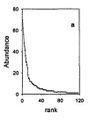
Fig. 2a. The rank-abundance plot (see also Fig. 4.)
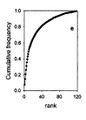
Fig. 2b. The [math]k[/math]-dominance plot
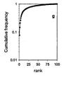
Fig. 2c. The Lorenzen curve
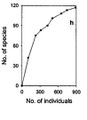
Fig. 2d. The collector’s curve
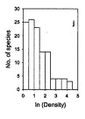
Fig. 2e. The species-abundance plot


Species-abundance models[3]
Species-abundance distributions (SADs) describe the distribution of population densities of all the species in a community. They are intermediate-complexity descriptors of a community's diversity: more informative than species richness but less detailed than a list of species and their abundances. The universally observed pattern is that most species in a community are rare, while a few are common, with abundances spanning orders of magnitude[16]. The most abundant species are generally considered core species, while rare species are occasional visitors from different adjacent habitats. The universal pattern of SADs suggests that general ecological principles must govern species abundance. Different models have been proposed based on various assumptions regarding the underlying ecological principles. No generally accepted model has emerged so far (2022)[17]. A few SADs that correspond to distributions commonly observed in ecosystems are presented below.
The log-series distribution
The log-series index [math]\alpha\,[/math] is a parameter of the log-series model that was derived by Fisher et al (1943[18]) from statistical arguments for very heterogeneous communities. The parameter [math]\alpha\,[/math] is a characteristic of the community and independent of sample size. It describes the way in which the individuals are divided among the species, which is a measure of diversity. The attractive properties of this diversity index are: it provides a good discrimination between sites, it is not very sensitive to density fluctuations and it is normally distributed such that confidence limits can be attached to [math]\alpha\,[/math]. Several different assumptions regarding biological dynamics can result in a log-series species-abundance distribution. The log series model is most successful in describing small numbers of species in succession communities, or in very harsh environments, but less adequate for larger areas, higher diversity or higher number of individuals[19].
The log series takes the form:
[math]\alpha\,x \, , \quad \Large\frac{\alpha\, x^2}{2} \, , \frac{\alpha\, x^3}{3} , \, …..\, , \frac{\alpha\, x^{n_S}}{n_S} \qquad[/math] or [math]\qquad s(j)= \Large\frac{\alpha\, x^j}{j} \normalsize , \; j=1, …, n_S , \qquad (11)[/math]
where [math]s(j)[/math] is the number of species present with [math]j[/math] individuals in the sampled community. Since, according to the log-series model, [math]0 \lt \,x \lt 1[/math] and [math]\alpha\,[/math] and [math]\,x[/math] are presumed to be constant, the expected number of species will be the highest for the first abundance class comprising a single individual. The total number of species [math]S= \sum_{j=1}^{n_S} s(j)=\alpha \sum_{j=1}^{n_S} (x^j / j) [/math] for a large sample with many species can be approximated by
[math]S \approx \alpha \sum_{j=1}^{\infty} x^j / j = - \alpha \, \ln(1-x) . \qquad (12)[/math]
The total number of individuals [math] N \ = \sum_{j=1}^{n_S} j s(j) = \alpha \sum_{j=1}^{n_S} x^j [/math] can under certain conditions be approximated by
[math] N \approx \alpha \sum_{j=1}^{\infty} x^j = \alpha \, x / (1-x). \qquad (13)[/math]
The values of [math]\,x[/math] and [math]\alpha[/math] can be estimated from these two equations (under the condition [math]x^{n_S} \lt \lt 1[/math]) by counting the total numbers [math]N[/math] and [math]S[/math] in the sample. It should be noted that, unless the number of species increases linearly with the sample size, the parameter [math]x[/math] depends on the sample size. The distribution over species thus changes with sample size.
The value of [math]x[/math] is usually very close to 1, such that [math]n_S \, (1-x) \lt \lt 1[/math]. In this case the Shannon-Wiener index can be approximated by [math]H' \approx \ln(\alpha)[/math], see appendix A3.
The log-normal distribution
Preston [20] first suggested to use a log-normal distribution for the description of species-abundances distributions. This is a normal (Gaussian) distribution for the parameter [math]y=\ln(n)[/math], the logarithm of the species abundance [math]n[/math] (= the number of individuals belonging to a particular species). Samples are considered with a large number of species and a large number of individuals. The log-normal distribution allows variation of [math]n[/math] from 0 to infinity; the corresponding values of [math]y[/math] are in the range [math][-\infty, +\infty][/math]. The distribution specifies the number of species [math]s(y)dy[/math] that may be expected with abundances [math]n[/math] in the interval [math][y,y+dy][/math]; it is given by
[math]s(y)dy = \Large\frac{S}{\sigma \sqrt{2\pi}}\normalsize \, \exp(-\Large\frac{(y-\mu)^2}{2 \sigma^2}\normalsize) \, dy , \qquad (14)[/math]
where [math]S[/math] is the total number of species and where [math]\mu[/math] and [math]\sigma[/math] are related to the average number of individuals per species and to the variance,
[math]\overline{n} = \Large\frac{N}{S}\normalsize = \exp(\mu + ½ \sigma^2) , \qquad \overline{(n-\overline{n})^2} = (\exp(\sigma^2) – 1)\, \exp(2 \mu +\sigma^2) . \qquad (15)[/math]
Contrary to the log-series distribution (Eq. 11), the log-normal distribution does not assume that species with the lowest abundance are most numerous. The log-normal distribution appears to be most appropriate for describing stable many-species communities, or sets of rapidly reproducing opportunist species.
Magurran and Henderson (2003[21]) explain the difference between the log-series distribution and the log-normal distribution as follows, based on a long-term (21-year) data set, from an estuarine fish community: "The ecological community can be separated into two components. Core species, which are persistent, abundant and biologically associated with estuarine habitats, are log normally distributed. Occasional species occur infrequently in the record, are typically low in abundance and have different habitat requirements; they follow a log-series distribution. These distributions are overlaid, producing the negative skew that characterizes real data sets." This is illustrated in Fig. 3.

The species-abundance distribution Eq. (14) can also be written as a rank-abundance distribution:
[math]n_i = \Large\frac{N}{S}\normalsize \exp(- \sigma^2/2 + \sqrt{2} \sigma erf^{(-1)}(1-2i/S )) , \qquad (16) [/math]
where [math]n_i[/math] is the abundance of species [math]i[/math] (species ranked in order of decreasing abundance) and where [math] erf^{(-1)}[/math] is the inverse error function, [math]erf^{(-1)}(erf(x))=x, \quad erf(x)=\Large\frac{2}{\sqrt{\pi}}\normalsize \int_0^x e^{-y^2}.[/math]
The Shannon-Wiener index for the log-normal distribution (Eq. 16) is given by
[math]H' \approx \ln(S) - \Large\frac{\sigma^2}{2}\normalsize . [/math]
The biodiversity index increases (i.e. the biodiversity increases) with increasing number of species [math]S[/math]. The index also increases when [math]\sigma[/math] decreases; when all species have similar abundance (high evenness = small [math]\sigma[/math]), the biodiversity is high.

The niche preemption model or the geometric model
This model assumes that a species preempts a fraction [math]k[/math] of a limiting resource, a second species the same fraction [math]k[/math] of the remainder and so on. If the abundances are proportional to their share of the resource, the rank-abundance distribution is given by geometric series (see appendix A4):
[math]\Large\frac{n_i}{N}\normalsize=\Large\frac{k(1-k)^{(i-1)}}{1-(1-k)^S}\normalsize , \qquad (17)[/math]
where [math]S[/math] is the number of the species in the community. For large values of [math]S[/math] this distribution depends only on the parameter [math]k[/math]. In this case the Shannon-Wiener index is given by [math]H' \approx -((1-k)/k) \ln(1-k) -\ln(k)[/math]. For small values of [math]k[/math] the index is large (high biodiversity) and for values of [math]k[/math] close to 1 the index is close to zero (low biodiversity).
The geometric model gives a straight line on a plot of log abundance against rank (species sequence), see Fig. 4. It is not very often found in nature, only in early successional stages or in species poor environments[15]. If the fraction [math]k[/math] is allowed to vary randomly, the geometric model becomes equivalent to the log series model of species abundance.
The broken-stick model or the negative exponential distribution
In this model a limiting resource is compared with a stick, broken in [math]S[/math] parts at [math]S-1[/math] randomly located points. The length of the parts is taken as representative for the density of the [math]S[/math] species subdividing the limiting resource. If the species are ranked according to abundance, the expected abundance [math]n_i[/math] of species [math]i[/math] is given by[22]:
[math]\Large\frac{n_i}{N}\normalsize= \Large\frac{1}{S}\normalsize \sum_{j = i}^S \frac{1}{j} . \qquad (18)[/math]
This distribution satisfies the condition [math]N = \sum_{i=1}^S n_i [/math]. The dependence on the single parameter [math]S[/math] is weak for large values of [math]S[/math]. For large values of [math]S[/math] the Shannon-Wiener index is close to [math]H' \approx ln(S)[/math].
The broken stick-model is most applicable to communities of a few taxonomically similar species, in a homogenous environment, between which a single overriding survival requirement is more or less equally divided. The negative exponential distribution is not often found in nature; it describes a fairly even distribution of individuals over species (Fig. 4) which is rare in natural communities[15].
Interpretation of observed species-abundance distributions
Species-abundance distributions (SADs) provide better information on ecological community characteristics than simple diversity indices for comparing communities in a management context. SADs enable relatively quick assessments of ecosystem health and the success of management interventions aimed at mitigating the effects of disturbance. Analysis of the SAD over time provides managers with early warning signals of the effects of disturbance on ecological communities[23].
For the interpretation of observed species abundance distributions, it is important that every individual of a given species is equally likely to be observed when the community is sampled, that observing each individual is an independent event, and the population remains unchanged during sampling. The scale and resolution of the sampling must be appropriate to the purpose of the study, and relevant abiotic factors must be included in the survey[24]. For example, increasing a sample to include a broader range of taxa may result in a multimodal SAD, which combines several unimodal SADs, each with its own set of parameters[19].
The species-abundance distributions determined from 'small' samples (abundances [math]n[/math] substantially less than 100) are generally biased. The reason is that the spatial distribution of species is not uniform. Clustered distributions lead to the greatest bias. In the case of a statistical random distribution of a species with an expected abundance of [math]n[/math] individuals in the sampled area, the probability to find an abundance [math]m \ne n[/math] for this species is given by the Poisson distribution [math]P_n(m)=\exp(-n) \, n^m \, / (m! P_{n,N})[/math]. [math]P_{n,N}[/math] is a normalization factor to ensure that [math]\sum_{m=1}^N P_n(m)=1[/math]. If [math]s(n)dn/S[/math] is interpreted as the expected probability to find a species with abundance in the range [math] [n- ½dn, n+ ½dn] [/math] in large samples, then in small samples one will find the species-abundance distribution [math]\hat s(n)=\sum_{m=1}^N P_n(m) s(m)[/math] instead of the expected distribution [math]s(n)[/math]. If the abundance [math]n[/math] is large, the Poisson distribution is strongly peaked around [math]m=n[/math], which implies [math]\hat s(n) \approx s(n) [/math]. If the species abundance [math]s(n)[/math] is lognormally distributed, then the observed species abundance [math]\hat s(n)[/math] follows a so-called Poisson log-normal distribution.
Appendix A1
The Shannon-Wiener diversity index is a measure of the information (in fact, the 'lack of information', or 'uncertainty' or 'information entropy') represented by a sample, where information is defined as the minimum length of a string of digits necessary to describe the sample. The minimum length of a string of (binary) digits to describe a number is proportional to the logarithm of this number. All the different ways in which [math]N[/math] individuals can be distributed in numbers [math]n_1, n_2, …, n_S[/math] for the species [math]1, 2, …., S[/math] are equivalent and thus provide no additional information about the sample. With this definition, a measure of the information entropy in a large sample is given by the logarithm of the number [math]P[/math] of all different permutations of individuals that give the same distribution of individuals over species. If [math]P[/math] is large, the sample can be ordered in many distinct equivalent ways and thus has a low information content (= high information entropy = high diversity). This is the case, for example, if all [math]N[/math] individuals in a sample belong to different species. The number of equivalent distinct permutations is then equal to [math]P=N![/math] (the first individual in an ordered sample can be chosen in [math]N[/math] ways, the second in [math]N-1[/math] ways and so on). If all the individuals belong to the same species there are no distinct equivalent permutations, i.e. [math]P=1[/math]. If there are [math]n_1[/math] individuals of species 1, [math]n_2[/math] individuals of species 2, and so on, then the number of equivalent distinct permutations is [math]P = N!/(n_1! \times n_2! \times . . . . \times n_S!)[/math]. Taking the natural logarithm gives [math]N \times[/math] the Brillouin index [math]H[/math]. Assuming that the numbers [math]N, n_1, n_2, ….[/math] are very large, one can approximate [math]\ln(n_i!) \approx n_i\, \ln(n_i) [/math]. This gives [math]\ln(P) \approx N \, \ln(N) - n_1 \, \ln(n_1) - n_2\, \ln(n_2) - …..- n_S \, \ln(n_S) [/math]. For large representative samples the probability of occurrence of species [math]i[/math] is given by [math]p_i=n_i/N[/math]. We further have [math]\sum_{i=1}^{S} p_i=1[/math]. Substitution gives [math]\ln(P) \approx -N \sum_{i=1}^{S} p_i \, \ln(p_i)[/math], which is [math]N \times[/math] the Shannon-Wiener index [math]H'[/math]. Division by [math]N[/math] makes the index independent of the sample size.
Another interpretation of the Shannon-Wiener index is: the mean number of digits required for describing the probability [math]p_i[/math] to find [math]n_i[/math] individuals of species [math]i[/math] in the sample of [math]N[/math] individuals. The number of digits for describing the probability [math]p_i[/math] is proportional to [math]-\ln(p_i)[/math] (the rarer the species, the smaller [math]p_i[/math] and the more digits are needed). The mean is obtained by taking the weighted sum of the number of digits: [math]H'= - \sum_{i=1}^S p_i \ln(p_i)[/math].
Appendix A2
Take [math]a=1+\epsilon[/math] and [math]\epsilon \to 0[/math], then [math]p_i^a \to p_i+\epsilon \large\frac{d}{d \epsilon} p_i^{1+\epsilon}\normalsize \approx p_i + \epsilon p_i \ln p_i[/math]. Because [math]\sum_{i=1}^S p_i = 1[/math], we have
[math]H_1 = \lim_{\epsilon \to 0} (1 + \epsilon \sum_{i=1}^S p_i \ln p_i)^{-1/\epsilon} = \exp(-\sum_{i=1}^S p_i \ln p_i)[/math].
Appendix A3
The conversion of the species-abundance distribution Eq. (11) into the rank-abundance distribution gives [math](n_i, x_i), \; i=1, …., n_S[/math], with [math]n_i=n_S+1-i, \quad x_i=\alpha \sum_{j=n_S+1-i}^{n_S} (x^j/j)[/math]. Summation over all species gives [math]N=\sum_{i=1}^{n_S} n_i \Delta x_i[/math], with [math]\Delta x_i=x_i-x_{i-1}=\alpha x^j/j, \; j=n_S+1-i, \; x_0=0[/math].
The Shannon-Wiener index is given by [math]H'=- \sum_{i=1}^{n_S} \Delta x_i (n_i/N) \ln(n_i/N)=\ln(N)-(\alpha/N)\sum_{j=1}^{n_S} x^j \ln(j)[/math]. Assuming [math]n_S\gt \gt 1[/math] and [math]n_S (1-x) \lt \lt 1[/math] we have [math]\alpha n_S \approx N[/math] and [math]\sum_{j=1}^{n_S} x^j \ln(j) \approx \sum_{j=1}^{n_S} \ln(j) = \ln(n_S!) \approx n_S \ln(n_S) \approx (N/ \alpha)(\ln(N)-\ln(\alpha))[/math]. Substitution yields [math]H' \approx \ln(\alpha)[/math].
Appendix A4
According to the assumptions underlying the model, the numbers [math]\, n_1, n_2, …., n_S \, [/math] of species [math]\, 1, 2, …., S \,[/math] are
[math]n_1=Ck, \; n_2= Ck(1-k), \; n_3=Ck(1-k-k(1-k))=Ck(1-k)^2, …., \; n_S=Ck(1-k)^{(S-1)} [/math].
We have [math]N = \sum_{i=1}^S n_i = Ck\sum_{i=1}^S (1-k)^{(i-1)} = C(1-(1-k)^S) [/math], hence [math]C=\Large\frac{N}{1-(1-k)^S}[/math].
See also
- Marine Biodiversity
- Biodiversity and Ecosystem function
- Biological Trait Analysis
- Wikipedia article Diversity index
Further reading
- Magurran, A. E. 2004. Measuring biological diversity, Blackwell Publishing: Oxford, UK. 256 p
References
- ↑ [\http://en.wikipedia.org/wiki/Biodiversity#Measurement_of_biodiversity Wikipedia article Measurement of biodiversity
- ↑ Whittaker, R.H. 1972. Evolution and measurement of species diversity. Taxon 21: 213-251
- ↑ 3.0 3.1 Magurran, A. E. 2004. Measuring biological diversity, Blackwell Publishing: Oxford, UK. 256 p
- ↑ Clifford H.T. and Stephenson W. 1975. An introduction to numerical classification. London: Academic Express.
- ↑ Whittaker R.H. 1977. Evolution of species diversity in land communities. Evolutionary Biol. 10: 1-67
- ↑ Shannon C. E. and Weaver W. 1949. The mathematical theory of communication. Urbana, IL: University of Illinois Press.
- ↑ 7.0 7.1 Pielou E.C. 1975. Ecological diversity. New York: Wiley Interscience.
- ↑ Pielou E.C. 1969. An introduction to mathematical ecology. New York: Wiley.
- ↑ Simpson E.H. 1949. Measurement of diversity. Nature 163: 688.
- ↑ Pielou, E.C. 1966. The measurement of diversity in different types of biological collection. Journal of Theoretical Biology 13: 131–144
- ↑ Hill, M.O. 1973. Diversity and evenness: a unifying notation and its consequences. Ecology 54: 427–473
- ↑ 12.0 12.1 Warwick R.M. and Clarke K.R. 2001. Practical measures of marine biodiversity based on relatedness of species. Oceanogr. Mar. Biol. Ann. Rev. 39: 207-231
- ↑ Clarke K.R. and Warwick R.M. 1998. A taxonomic distinctness index and its statistical properties Journal of Applied Ecology 35 (4): 523-531
- ↑ Petchey O.L. and Gaston K.J. 2002. Functional diversity (FD), species richness and community composition. Ecology letters Vol. 5 (3): 402-411
- ↑ 15.0 15.1 15.2 Heip, C.H.R., Herman, P.M.J. and Soetaert, K. 1998. Indices de diversité et régularité. [Indices of diversity and evenness]. Océanis (Doc. Océanogr.) 24(4): 67-87
- ↑ McGill, B.J., Etienne, R.S., Gray, J.S., Alonso, D., Anderson, M.J., Benecha, H.K., Dornelas, M., Enquist, B.J., Green, J.L., He, F., Hurlbert, A.H., Magurran, A.E., Marquet, P.A., Maurer, B.A., Ostling, A., Soykan, C.U., Ugland, K.I. and White, E.P. 2007. Species abundance distributions: moving beyond single prediction theories to integration within an ecological framework. Ecology Letters, 10, 995–1015
- ↑ Koffel, T., Umemura, K., Litchman, E. and Klausmeier, C.A. 2022. A general framework for species-abundance distributions: Linking traits and dispersal to explain commonness and rarity. Ecology letters. Online version published 14 September 2022
- ↑ Fisher, R. A., Corbet, A. S. and Williams, C. B. 1943. The relation between the number of species and the number of individuals in a random sample of an animal population. Journal of Animal Ecology 12: 42-58
- ↑ 19.0 19.1 Antao, L.H., Magurran, A.E. and Dornelas, M. 2021. The Shape of Species Abundance Distributions Across Spatial Scales. Front. Ecol. Evol. 9:626730
- ↑ Preston, F.W. 1948. The commonness and rarity of species. Ecology 29: 254–283
- ↑ 21.0 21.1 Magurran, A.E. and Henderson, P.A. 2003. Explaining the excess of rare species in natural species abundance distributions. Nature 422: 714–716
- ↑ McArthur, R.H. 1957. On the relative abundance of bird species. Proc. Natl. Acad. Sci. USA 43: 293-295
- ↑ Matthews, T.J. and Whittaker, R.J. 2015. On the species abundance distribution in applied ecology and biodiversity management. Journal of Applied Ecology 52: 443–454
- ↑ Austin, M. 2007. Species distribution models and ecological theory: A critical assessment and some possible new approaches. Ecological modelling 200: 1-19
Please note that others may also have edited the contents of this article.
|