|
|
| (7 intermediate revisions by the same user not shown) |
| Line 1: |
Line 1: |
| − | Tidal bore dynamics
| + | {{Review |
| | + | |name=Job Dronkers|AuthorID=120| |
| | + | }} |
| | | | |
| − | A tidal bore is the ultimate stage of distortion of a tidal wave that propagates upstream a river. This article describes the processes involved in this ultimate stage of tidal wave deformation and the modelling of these processes. For an introduction to the topic of tidal wave deformation the reader is referred to the article [[Tidal asymmetry and tidal basin morphodynamics]].
| |
| | | | |
| | + | '''Resilience and resistance''' |
| | | | |
| − | ==Introduction==
| |
| | | | |
| | + | {{Definition|title=Resistance |
| | + | |definition= The capacity to weather a disturbance without loss (Lake 2013<ref name=L>Lake, P.S. 2013. Resistance, Resilience and Restoration. Ecological Management and Restoration 14: 20-24</ref>). }} |
| | | | |
| − | {| style="border-collapse:collapse; font-size: 12px; background:ivory;" cellpadding=5px align=right width=50%
| |
| − | |+ Table 1. Estuaries and rivers with substantial tidal bores (bore height of half a meter up to several meters).
| |
| − | |- style="font-weight:bold; font-size: 11px; text-align:center; background:lightblue"
| |
| − | ! width="25% style=" border:1px solid blue;"| Estuary/river name
| |
| − | ! width="5% style=" border:1px solid bleu;"| Maximum tidal range [m]
| |
| − | ! width="20% style=" border:1px solid blue;"| Tide gauge location
| |
| − | ! width="10% style=" border:1px solid blue;"| Country
| |
| − | |-
| |
| − | | style="border:2px solid lightblue; font-size: 10px; text-align:center"| Shannon River
| |
| − | | style="border:2px solid lightblue; font-size: 10px; text-align:center"| 5.6
| |
| − | | style="border:2px solid lightblue; font-size: 10px; text-align:center"| Shannon
| |
| − | | style="border:2px solid lightblue; font-size: 10px; text-align:center"| Ireland
| |
| − | |-
| |
| − | | style="border:2px solid lightblue; font-size: 10px; font-size: 10px; font-size: 10px; text-align:center"| Humber,Trent
| |
| − | | style="border:2px solid lightblue; font-size: 10px; font-size: 10px; text-align:center"| 8.3
| |
| − | | style="border:2px solid lightblue; font-size: 10px; text-align:center"| Hull
| |
| − | | style="border:2px solid lightblue; font-size: 10px; text-align:center" rowspan="8"| UK
| |
| − | |-
| |
| − | | style="border:2px solid lightblue; font-size: 10px; text-align:center"| Great Ouse
| |
| − | | style="border:2px solid lightblue; font-size: 10px; text-align:center"| 7.4
| |
| − | | style="border:2px solid lightblue; font-size: 10px; text-align:center"| King's Lynn
| |
| − | |-
| |
| − | | style="border:2px solid lightblue; font-size: 10px; text-align:center"| Severn
| |
| − | | style="border:2px solid lightblue; font-size: 10px; text-align:center"| 12
| |
| − | | style="border:2px solid lightblue; font-size: 10px; text-align:center"| Portishead
| |
| − | |-
| |
| − | | style="border:2px solid lightblue; font-size: 10px; text-align:center"| Dee
| |
| − | | style="border:2px solid lightblue; font-size: 10px; text-align:center"| 9.8
| |
| − | | style="border:2px solid lightblue; font-size: 10px; text-align:center"| Flint
| |
| − | |-
| |
| − | | style="border:2px solid lightblue; font-size: 10px; text-align:center"| Mersey
| |
| − | | style="border:2px solid lightblue; font-size: 10px; text-align:center"| 10
| |
| − | | style="border:2px solid lightblue; font-size: 10px; text-align:center"| Liverpool
| |
| − | |-
| |
| − | | style="border:2px solid lightblue; font-size: 10px; text-align:center"| Ribble
| |
| − | | style="border:2px solid lightblue; font-size: 10px; text-align:center"| 10.2
| |
| − | | style="border:2px solid lightblue; font-size: 10px; text-align:center"| Lytham
| |
| − | |-
| |
| − | | style="border:2px solid lightblue; font-size: 10px; text-align:center"| Morecambe bay, Nith River, River Kent
| |
| − | | style="border:2px solid lightblue; font-size: 10px; text-align:center"| 10.9
| |
| − | | style="border:2px solid lightblue; font-size: 10px; text-align:center"| Morecambe
| |
| − | |-
| |
| − | | style="border:2px solid lightblue; font-size: 10px; text-align:center"| River Eden
| |
| − | | style="border:2px solid lightblue; font-size: 10px; text-align:center"| 10.3
| |
| − | | style="border:2px solid lightblue; font-size: 10px; text-align:center"| Silloth
| |
| − | |-
| |
| − | | style="border:2px solid lightblue; font-size: 10px; text-align:center"| Seine
| |
| − | | style="border:2px solid lightblue; font-size: 10px; text-align:center"| 8.5
| |
| − | | style="border:2px solid lightblue; font-size: 10px; text-align:center"| Honfleur
| |
| − | | style="border:2px solid lightblue; font-size: 10px; text-align:center" rowspan="4"| France
| |
| − | |-
| |
| − | | style="border:2px solid lightblue; font-size: 10px; text-align:center"| Canal de Carentan
| |
| − | | style="border:2px solid lightblue; font-size: 10px; text-align:center"| 7
| |
| − | | style="border:2px solid lightblue; font-size: 10px; text-align:center"| Carentan
| |
| − | |-
| |
| − | | style="border:2px solid lightblue; font-size: 10px; text-align:center"| Baie du Mont Saint Michel – Sélune River
| |
| − | | style="border:2px solid lightblue; font-size: 10px; text-align:center"| 14
| |
| − | | style="border:2px solid lightblue; font-size: 10px; text-align:center"| Granville
| |
| − | |-
| |
| − | | style="border:2px solid lightblue; font-size: 10px; text-align:center"| Garonne, Dordogne
| |
| − | | style="border:2px solid lightblue; font-size: 10px; text-align:center"| 6
| |
| − | | style="border:2px solid lightblue; font-size: 10px; text-align:center"| Bordeaux
| |
| − | |-
| |
| − | | style="border:2px solid lightblue; font-size: 10px; text-align:center"| Pungue
| |
| − | | style="border:2px solid lightblue; font-size: 10px; text-align:center"| 7
| |
| − | | style="border:2px solid lightblue; font-size: 10px; text-align:center"| Beira
| |
| − | | style="border:2px solid lightblue; font-size: 10px; text-align:center"| Mozambique
| |
| − | |-
| |
| − | | style="border:2px solid lightblue; font-size: 10px; text-align:center"| Qiantang
| |
| − | | style="border:2px solid lightblue; font-size: 10px; text-align:center"| 5
| |
| − | | style="border:2px solid lightblue; font-size: 10px; text-align:center"| Ganpu
| |
| − | | style="border:2px solid lightblue; font-size: 10px; text-align:center"| China
| |
| − | |-
| |
| − | | style="border:2px solid lightblue; font-size: 10px; text-align:center"| Indus
| |
| − | | style="border:2px solid lightblue; font-size: 10px; text-align:center"| 4
| |
| − | | style="border:2px solid lightblue; font-size: 10px; text-align:center"| Port Muhammad Bin Qasim
| |
| − | | style="border:2px solid lightblue; font-size: 10px; text-align:center"| Pakistan
| |
| − | |-
| |
| − | | style="border:2px solid lightblue; font-size: 10px; text-align:center"| Hooghly
| |
| − | | style="border:2px solid lightblue; font-size: 10px; text-align:center"| 5.7
| |
| − | | style="border:2px solid lightblue; font-size: 10px; text-align:center"| Sagar Island
| |
| − | | style="border:2px solid lightblue; font-size: 10px; text-align:center"| India
| |
| − | |-
| |
| − | | style="border:2px solid lightblue; font-size: 10px; text-align:center"| Brahmaputra
| |
| − | | style="border:2px solid lightblue; font-size: 10px; text-align:center"| 5.7
| |
| − | | style="border:2px solid lightblue; font-size: 10px; text-align:center"| Chittagong
| |
| − | | style="border:2px solid lightblue; font-size: 10px; text-align:center"| Bangladesh
| |
| − | |-
| |
| − | | style="border:2px solid lightblue; font-size: 10px; text-align:center"| Sittaung
| |
| − | | style="border:2px solid lightblue; font-size: 10px; text-align:center"| 6.3
| |
| − | | style="border:2px solid lightblue; font-size: 10px; text-align:center"| Moulmein
| |
| − | | style="border:2px solid lightblue; font-size: 10px; text-align:center"| Myanmar
| |
| − | |-
| |
| − | | style="border:2px solid lightblue; font-size: 10px; text-align:center"| Batang Lupar River
| |
| − | | style="border:2px solid lightblue; font-size: 10px; text-align:center"| 5.6
| |
| − | | style="border:2px solid lightblue; font-size: 10px; text-align:center"| Kuching
| |
| − | | style="border:2px solid lightblue; font-size: 10px; text-align:center"| Sarawak
| |
| − | |-
| |
| − | | style="border:2px solid lightblue; font-size: 10px; text-align:center"| Kampar River
| |
| − | | style="border:2px solid lightblue; font-size: 10px; text-align:center"| 5.3
| |
| − | | style="border:2px solid lightblue; font-size: 10px; text-align:center"| Pulo Muda
| |
| − | | style="border:2px solid lightblue; font-size: 10px; text-align:center"| Sumatra
| |
| − | |-
| |
| − | | style="border:2px solid lightblue; font-size: 10px; text-align:center"| Hooghly
| |
| − | | style="border:2px solid lightblue; font-size: 10px; text-align:center"| 5.7
| |
| − | | style="border:2px solid lightblue; font-size: 10px; text-align:center"| Sagar Island
| |
| − | | style="border:2px solid lightblue; font-size: 10px; text-align:center"| India
| |
| − | |-
| |
| − | | style="border:2px solid lightblue; font-size: 10px; text-align:center"| Fly , Bamu, Turamu Rivers
| |
| − | | style="border:2px solid lightblue; font-size: 10px; text-align:center"| 4.2
| |
| − | | style="border:2px solid lightblue; font-size: 10px; text-align:center"| estuary
| |
| − | | style="border:2px solid lightblue; font-size: 10px; text-align:center"| West Papua
| |
| − | |-
| |
| − | | style="border:2px solid lightblue; font-size: 10px; text-align:center"| Styx
| |
| − | | style="border:2px solid lightblue; font-size: 10px; text-align:center"| 6.4
| |
| − | | style="border:2px solid lightblue; font-size: 10px; text-align:center"| Mackay, Queensland
| |
| − | | style="border:2px solid lightblue; font-size: 10px; text-align:center" rowspan="2"| Australia
| |
| − | |-
| |
| − | | style="border:2px solid lightblue; font-size: 10px; text-align:center"| Daly River
| |
| − | | style="border:2px solid lightblue; font-size: 10px; text-align:center"| 7.9
| |
| − | | style="border:2px solid lightblue; font-size: 10px; text-align:center"| estuary
| |
| − | |-
| |
| − | | style="border:2px solid lightblue; font-size: 10px; text-align:center"| Turnagain Arm, Knick Arm
| |
| − | | style="border:2px solid lightblue; font-size: 10px; text-align:center"| 7.9
| |
| − | | style="border:2px solid lightblue; font-size: 10px; text-align:center"| Anchorage
| |
| − | | style="border:2px solid lightblue; font-size: 10px; text-align:center"| Alaska
| |
| − | |-
| |
| − | | style="border:2px solid lightblue; font-size: 10px; text-align:center"| Bay of Fundy, Petitcodiac and Salmon rivers
| |
| − | | style="border:2px solid lightblue; font-size: 10px; text-align:center"| 16
| |
| − | | style="border:2px solid lightblue; font-size: 10px; text-align:center"| Truro
| |
| − | | style="border:2px solid lightblue; font-size: 10px; text-align:center"| Canada
| |
| − | |-
| |
| − | | style="border:2px solid lightblue; font-size: 10px; text-align:center"| Colorado River
| |
| − | | style="border:2px solid lightblue; font-size: 10px; text-align:center"| 7.7
| |
| − | | style="border:2px solid lightblue; font-size: 10px; text-align:center"| San Filipe
| |
| − | | style="border:2px solid lightblue; font-size: 10px; text-align:center"| Mexico
| |
| − | |-
| |
| − | | style="border:2px solid lightblue; font-size: 10px; text-align:center"| Amazon, Araguira, Guama, Capim and Mearim Rivers
| |
| − | | style="border:2px solid lightblue; font-size: 10px; text-align:center"| 3.4
| |
| − | | style="border:2px solid lightblue; font-size: 10px; text-align:center"| Macapa
| |
| − | | style="border:2px solid lightblue; font-size: 10px; text-align:center"| Brazil
| |
| − | |}
| |
| | | | |
| | + | {{Definition|title=Resilience |
| | + | |definition=(1) the capability to anticipate, prepare for, respond to, and recover from significant multihazard threats with minimum damage to social well-being, the economy, and the environment (sometimes called 'socio-ecological resilience')(Olsen et al. 2019<ref name=O>Olsson, S., Melvin, A. and Giles, S. (eds.) 2019. Climate change and ecosystems. Procs. Sackler Forum on Climate Change and Ecosystems, Washington, DC, November 8-9, 2018, organized by the National Academy of Sciences and The Royal Society</ref>); |
| | | | |
| − | When a tidal wave propagates upstream into an estuary its shape is progressively distorted. If the mean channel depth <math>D_0</math> is not much greater than the spring tidal range <math>2a</math> (same order of magnitude or a few times larger) and if the intertidal area is smaller than the tidal channel surface area, the high-water (HW) wave crest will propagate faster up-estuary than the low-water (LW) wave trough. The tidal rise period is shortened and the tidal wave is becoming steeper. If the tidal wave can propagate sufficiently far upstream the river without strong damping, the tidal wave front may become so steep that tidal rise corresponds to a water level jump – a so-called tidal bore.
| + | (2) the capability of a (socio-)ecological system to remain within a stability domain when subjected to environmental change, while continually changing and adapting yet remaining within critical thresholds (sometimes called 'general resilience') (Folke et al. 2010<ref name=F>Folke, C., Carpenter, S. R., Walker, B., Scheffer, M., Chapin, T. and Rockstrom, J. 2010. Resilience thinking: integrating resilience, adaptability and transformability. Ecology and Society 15(4): 20</ref>; Scheffer 2009<ref>Scheffer, M. 2009. Critical transitions in nature and society. Princeton University Press, Princeton, New Jersey, USA</ref>; Brand and Jax 2007<ref name=BJ>Brand, F.S. and K. Jax. 2007. Focusing the meaning(s) of resilience: resilience as a descriptive concept and a boundary object. Ecology and Society 12(1):23</ref>); |
| | | | |
| − | Table 1 gives an overview of estuaries and tidal rivers in which significant tidal bores have been observed. It can be concluded from the table that tidal bores often occur in megatidal zones - areas where the maximum tidal range is greater than 6 m. However, it appears that substantial tidal bores can also occur in areas where the tidal range is smaller, although this is the exception rather than the rule. This exception seems to be limited to tropical and subtropical countries. Rivers are generally shallower in these regions due to abundant supply of fine sediments. Another possible reason is the relative importance of K1 and O2 diurnal tidal components, which can combine with the semidiurnal M2 tide to yield persistent tidal asymmetry <ref>Hoitink, A.F.J., Hoekstra, P. and van Mare, D.S. 2003. Flow asymmetry associated with astronomical tides: Implications for residual transport of sediment. J.Geophys.Res. 108: 13-1 - 13-8</ref> (see also the article [[Ocean and shelf tides]]). However, for the rivers listed in Table 1 this does not seem to play an important role <ref>Song, D., X. H. Wang, A. E. Kiss, and Bao, X. 2011. The contribution to tidal asymmetry by different combinations of tidal constituents. J. Geophys. Res., 116, C12007</ref>.
| + | (3) the capacity to experience shocks while retaining essentially the same function, structure, feedbacks, and therefore identity (sometimes called 'ecological resilience') (Brand and Jax 2007<ref name=BJ/>; DEFRA 2019<ref name=DEFRA>Haines‐Young, R. and Potschin. M. (eds.) 2010. The Resilience of Ecosystems to Environmental Change (RECCE). Overview Report, 27 pp. Defra Project Code: NR0134</ref>), which is closely related to the concept of 'ecosystem resistance': the amount of disturbance that a system can withstand before it shifts into a new regime or an alternative stable state (Holling 1973<ref>Holling, C.S. 1973. Resilience and stability of ecological systems. Annual Rev. Ecol. Syst. 4: 1–23. doi: 10.1146/annurev.es.04.110173.000245</ref>; Gunderson 2000<ref>Gunderson, L.H. 2000. Ecological Resilience - in Theory and Application. Annual Review of Ecology and Systematics 31:425-439.</ref>); |
| | | | |
| − | Engineering works (weirs, dredging) during the past century have weakened or even completely suppressed tidal bores in many rivers, for example in the rivers Seine, Loire, Charente and Petitcodiac.
| + | (4) the capacity of an ecosystem to regain its fundamental structure, processes, and functioning (or remain largely unchanged) despite stresses, disturbances, or invasive species (e.g., Hirota et al., 2011<ref>Hirota,M., Holmgren,M., Van Nes, E. H, and Scheffer,M. 2011. Global resilience of tropical forest and savanna to critical transitions. Science 334: 232–235. doi: 10.1126/science.1210657</ref>; Chambers et al., 2014<ref>Chambers, J. C., Bradley, B. A., Brown, C. S., D’Antonio, C., Germino, M. J., Grace, J. B., et al. 2014. Resilience to stress and disturbance, and resistance to Bromus tectorum L. invasion in the cold desert shrublands of western North America. Ecosystems 7: 360–375. doi: 10.1007/s10021-013-9725-5</ref>; Pope et al., 2014<ref>Pope, K. L., Allen, C. R., and Angeler, D. G. 2014. Fishing for resilience. T. N. Am. Fisheries Soc. 143: 467–478. doi: 10.1080/00028487.2014.880735</ref>; Seidl et al., 2016<ref>Seidl, R., Spies, T. A., Peterson, D. L., Stephens, S. L., and Hick, J. A. 2016. Searching for resilience: addressing the impacts of changing disturbance regimes on forest ecosystem services. J. Appl. Ecol. 53 : 120–129. doi: 10.1111/1365-2664.12511</ref>), which can be measured by the time needed to recover its original state (sometimes called 'engineering resilience'<ref name=L>Lake, P.S. 2013. Resistance, Resilience and Restoration. Ecological Management and Restoration 14: 20-24</ref>). |
| | + | }} |
| | | | |
| − | Illustrations of tidal bores are shown in Fig. 1.
| |
| | | | |
| | | | |
| | + | ==Introduction== |
| | + | Coastal and marine ecosystems are affected by environmental disturbance at a variety of spatio-temporal scales. The organisms inhabiting these systems are adapted to such disturbance, either by being tolerant of these conditions or by playing a role in one or more of the successional stages that follow during ecosystem recovery. |
| | | | |
| − | ==Tidal bore formation==
| + | If all species in the system were tolerant to a particular perturbation, very little would change at the ecosystem level, and we could call the system resistant to this disturbance. However, often a disturbance, such as a temporary very low oxygen level, affects a substantial proportion of the organisms dramatically, either causing them to die, or forcing them to rapidly migrate to more favorable parts of the environment. Such an adverse disturbance could locally defaunate a certain volume in the pelagic or a certain area of hard or soft substrate. Such destruction at a local scale does not mean the end of local functioning. Usually organisms are available at a larger spatial scale that can re-colonize the affected area, according to their particular tolerances and abilities to favorably affect their local environment. |
| − | | |
| − | The analysis of nonlinear tidal wave transformation in estuaries, in terms of tidal forcing at the estuary mouth and large-scale geometrical properties of the channel, has received considerable attention (see [[Tidal asymmetry and tidal basin morphodynamics]]). By contrast, the extreme nonlinear tidal-wave case where tidal bores form is much less studied.
| |
| − | | |
| − | The formation of tidal bores is mainly governed by the progressive distortion of the tidal wave as it propagates up the estuary. This extreme nonlinear deformation of the tidal wave occurs under special conditions, in particular<ref name=B15>Bonneton, P., Bonneton, N., Parisot, J-P. and Castelle, B. 2015. Tidal bore dynamics in funnel-shaped estuaries. J. Geophys. Res.: Ocean 120: 923-941. DOI: 10.1002/2014JC010267</ref> <ref name=R>Rousseaux, G., Mougenot, J. M., Chatellier, L., David, L. and Calluaud, D. 2016. A novel method to generate tidal-like bores in the laboratory. European Journal of Mechanics-B/Fluids 55:31-38</ref>:
| |
| − | *a large tidal amplitude <math>a</math>,
| |
| − | * a long, shallow and convergent channel.
| |
| − | | |
| − | River flow and river-bed slope also influence tidal bore formation. River flow contributes to tidal wave deformation by enhancing the longitudinal velocity gradient and river-bed slope by upstream reduction of the water depth. However, river flow and river-bed slope also contribute to tidal wave damping and thus oppose tidal bore formation <ref> Horrevoets, A. C., Savenije, H. H. G., Schuurman, J. N. and Graas, S. 2004. The influence of river discharge on tidal damping in alluvial estuaries. Journal of Hydrology 294: 213-228</ref>. The latter effect usually dominates. Observations show that the tidal bore in the Garonne and Dordogne (France) is suppressed at high river runoff<ref name=B16>Bonneton, P., Filippini, A.G., Arpaia, L., Bonneton, N. and Ricchiuto, M. 2016. Conditions for tidal bore formation in convergent alluvial estuaries. Estuarine, Coastal and Shelf Science. 172: 121-127</ref>. A similar effect is observed in the Daly estuary by Wolanski et al. (2006), who relate the occurrence of the tidal bore at low river discharge to the small water depth during such conditions. The opposite effect is reported for the Guamá-Capim river system near the mouth of the Amazon River, where tidal bores are observed only at high river discharges, in conjunction with high equinoctial tides<ref>Freitas, P.T.A., Silveira, O.F.M. and Asp, N.E. 2012. Tide distortion and attenuation in an Amazonian tidal river. Brazilian journal of oceanography, 60: 429-446</ref>.
| |
| − | | |
| − | | |
| − | [[Image:Seine-Qiangtang.jpg|center|700px|thumb|Figure 1. Many natural estuaries have large shoals in the mouth zone. These so-called mouth bars strongly enhance distortion of the tidal wave entering the estuary. Left image: Tidal bore in the Seine River around 1960, before the mouth bar was dredged. Right image: Tidal bore in the Qiangtang estuary, where a large mouth bar is still present (https://en.wikipedia.org/wiki/Qiantang_River ).]]
| |
| − | | |
| − | | |
| − | Although most studies of tidal bore formation have focused on estuary-river systems with gradual bed slopes, there is strong evidence that steep gradients in the mean depth may induce tidal bore formation. This phenomenon is well known for tsunami waves propagating onto the shoreface or for swell waves collapsing on the beach. Observations show that tidal bores often develop in shallow rivers that discharge from the higher upstream zone into a broad estuary. If the tidal wave has already acquired sufficient asymmetry when travelling through the estuary, a tidal bore develops when the tidal wave surges into the shallow river. The different stages of tidal bore formation are sketched in Fig. 2 <ref name=L>Lynch, D.K. 1982. Tidal bores. Scientific American 247: 146-157</ref>. In this case river discharge is favorable to tidal bore development. Fig. 3 shows the sharp increase in the current velocity and suspended sediment concentration recorded in the megatidal Baie du Mont Saint Michel at spring tide when the tidal flood wave enters the tidal flat area of the landward inner basin.
| |
| − | | |
| − | | |
| − | [[Image:TidalFlatBoreFormation-MorecambeBay.jpg |center|900px|thumb|Figure 2. Left panels, 1-4. Schematic representation of successive stages of tidal bore development when the tidal flood wave propagates from a tidal basin into a shallow upstream intertidal area. Adapted from Lynch(1982) <ref name=L> </ref>. Right panel: Tidal bore spilling over the intertidal mudflats of the megatidal Morecambe bay. Photo credit Arnold Price.]]
| |
| − | | |
| − | | |
| − | | |
| − | [[Image:SedimentTideBoreSaintMichel.jpg|center|900px|thumb|Figure 3. Tide elevation <math>\small \zeta</math> (above the dry bed), current velocity <math>\small u</math> and suspended sediment concentration <math>\small c</math> during springtide on a tidal flat in the Baie du Mont Saint Michel. The measurements started when the tidal flat at the measuring station was (almost) dry, just before the tidal bore spilled over the tidal flat. A rapid rise of the current velocity was recorded when the bore arrived. The suspended sediment concentration (mainly fine silty sand) peaked sharply at the passage of the bore front and quickly felt down afterwards. During the remaining flood period and during ebb the suspended sediment concentrations were much lower. The measurements illustrate the strong bottom stirring and sediment resuspension produced by the turbulent bore front, which significantly contributes to landward sediment transport and tidal basin infill <ref name=M>Migniot, C. 1998. Mission Mont Saint Michel - Synthèse des connaissances hydro-sédimentaires. Direction Départementale de l'Equipement de la Manche, 111pp.</ref>. A video of the arrival of the tidal bore can be viewed by clicking [https://www.youtube.com/watch?v=waeS1MvhT9M here]. The photo at the right is a still from the video.]]
| |
| − | | |
| − | | |
| − | | |
| − | | |
| − | ==Propagation of tidal bores==
| |
| − | | |
| − | [[Image:TidalBorePropagation.jpg|right|400px|thumb|Figure 4: Schematic representation of a hydraulic jump propagating with velocity <math>c</math> in a moving frame. In this frame moving with velocity <math>c</math> the hydraulic jump appears stationary; time derivatives are zero. The corresponding mass and momentum balance equations from which the propagation characteristics can be derived are indicated in the figure. The symbols used stand for: <math>u</math>= flow velocity in a fixed frame, <math>v</math>= flow velocity in the moving frame, <math>D</math>= water depth, <math>g</math>=gravitational acceleration; subscripts 1 and 2 indicate upstream and downstream conditions, respectively.]]
| |
| − | | |
| − | Nonlinear processes become increasingly important in the final stages of bore development. These processes can no longer be analyzed with analytical methods, but only with numerical simulation models. The hydrostatic long-wave equations cannot be applied to describe the emergence of a breaking tidal wave. Non-hydrostatic effects must be taken into consideration. This will be discussed further in the next sections.
| |
| − | | |
| − | A bore is a propagating transition between two streams of water depths <math>D_1</math> and <math>D_2</math> with speed <math>c=(D_2u_2-D_1u_1)/ (D_2-D_1)</math>, where <math>D_1 < D_2</math>. Once such a hydraulic jump has developed, its propagation characteristics can be derived from the mass and momentum balance equations, see Fig. 4. By eliminating <math>v_1=c-u_1</math> or <math>v_2=c-u_2</math> from these equations two equivalent expressions can be derived for the height of the tidal bore:
| |
| − | | |
| − | <math>\Delta D= \Large \frac{D_1}{2} [\normalsize -3 + \sqrt{1 + 8 F_1^2} \Large ] \normalsize = \Large \frac{D_2}{2} [\normalsize 3 - \sqrt{1 + 8 F_2^2} \Large ] \normalsize, \quad \quad (1)</math>
| |
| − | | |
| − | where <math>\Delta D=D_1 -D_2</math> is the bore height and the Froude numbers are given by
| |
| − | | |
| − | <math>F_1^2 = \Large \frac{v_1^2}{g D_1}\normalsize = \large \frac{D_2 (D_1+D_2)}{2 D_1^2} \normalsize , \quad F_2^2 = \Large \frac{v_2^2}{g D_2}\normalsize = \large \frac{D_1 (D_2+D_1)}{2 D_2^2} \normalsize . \quad \quad (2)</math>
| |
| − | | |
| − | For <math>\Delta D< 0.4 h_2</math> the tidal bore propagation speed <math>c</math> can be fairly well represented by
| |
| − | | |
| − | <math>c \approx \Large \frac{1}{2} \normalsize (c_1 + c_2) , \quad \quad (3)</math>
| |
| | | | |
| − | where <math> c_1 = u_1 + \sqrt{g D_1} , \quad c_2 = u_2 + \sqrt{g D_2}</math>.
| + | The term resilience has been defined in different ways, illustrated in the definition above. According to DEFRA (2019<ref name=DEFRA/>) there is limited consensus in the literature about how resilience can be characterized and assessed. The term resilience is sometimes used to represent some kind of normative proposition about what kinds of ecosystem characteristics are desirable or necessary in the context of sustainable development, reflecting particular cultural and philosophical assumptions<ref name=DEFRA/>. However, the resistance of an ecosystem (see the definition above) to changing conditions and the rate of recovery following some disruptive event are generally considered major components of resilience that can in principle be expressed in quantitative terms. |
| | | | |
| − | If the bore velocity <math> c </math> is equal to <math>c_2</math> (i.e. <math>F_2 = 1</math>) the bore height <math> \Delta D</math> is zero. Another requirement for a tidal bore is therefore <math>c < c_2</math> or <math>F_2 < 1</math> and <math>F_1 > 1</math>. Because <math>c_2</math> is the propagation speed of long-wave disturbances upstream of the bore, these disturbances (undulations) will catch up to the bore. A slowly propagating bore (<math>F_2 << 1</math>) will thus grow faster and become higher than a fast propagating bore (<math>F_1, F_2 </math> close to 1) <ref>Dronkers, J.J. 1964. Tidal computations in rivers and coastal waters. North-Holland Publ. Co., 518 pp.</ref>.
| + | Other attributes such as the capacity of ecosystems to transform and adapt in the face of environmental change (i.e. system's ability to re-organize itself) are more difficult to translate to practice. According to Dawson et al. (2010<ref name=D>Dawson, T.P., Rounsevell, M.D.A., Kluvankova‐Oravska, T., Chobotova V. and Stirling, A. 2010. Dynamic properties of complex adaptive ecosystems: implications for the sustainability of services provision. Biodiversity and Conservation 19: 2843‐2853</ref>), resilience concerns the response of ecosystems to changing environmental conditions and must be looked at alongside other additional dynamic features, namely durability, robustness and stability. These concepts can be defined as<ref name=D/>: |
| | + | * Durability: ability to cope with a chronic stress, but the source of this stress is endogenous; |
| | + | * Robustness: ability to recover or maintain the systems' social-ecological functions in the face of an external and chronic driver; |
| | + | * Stability: system’s tolerance to transient and endogenous shocks or disruptions. |
| | | | |
| | + | Both resistance and resilience cause an ecosystem to remain relatively unchanged when confronted to a disturbance, but in the case of resistance no internal re-organization and successional change is involved. In contrast, resilience implies that the system is internally re-organizing, perhaps through a mozaic of patches that are at different stages of re-assembly. System responses to changing environmental conditions are displayed schematically in Fig. 1, corresponding to different resilience characteristics. |
| | | | |
| | + | [[Image:ResilienceTrajectories.jpg|thumb|900px|center|Figure 1. Schematic representation of the trajectories of a (socio-)ecological system in a plane defined by the system state (fundamental structure, processes, and functioning - vertical axis) and the change of environmental conditions (horizontal axis), for different resilience characteristics (a, b, c, d). The initial state corresponds to the position on the graph at the vertical axis (zero change in environmental conditions). In all situations the ecosystem is assumed to collapse irreversibly (down to the horizontal axis) when the change in environmental conditions is much greater than the systems' resistance. The angle <math>\alpha</math> represents the rate at which the system recovers when the change in environmental conditions is reduced (small <math>\alpha</math> means slow recovery, large <math>\alpha</math> means fast recovery). Panel a: Resilience characterized by high resistance (definition 3) and slow recovery (definition 4). Panel b: Resilience characterized by low resistance and fast recovery. Panel c: Resilience characterized by a shift to an alternative stable system state. Panel d: Low resilience, characterized by low resistance and slow recovery.]] |
| | | | |
| − | ==Tidal bore characteristics==
| |
| | | | |
| − | In the previous section the tidal bore is represented by a hydraulic jump separating upstream and downstream regions of constant water depth. This simplification ignores the fact that energy loss occurs in the transition zone. Conservation of mass and momentum at the transition does not imply conservation of energy; there is a positive energy head loss
| + | When considering the potential effect of a certain type of disturbance it is thus useful to ask two questions: |
| | + | # Will the species of this system be able to tolerate it (implying resistance), and if not, |
| | + | # Is recovery possible through a successional trajectory, back to the same, or at least a desirable, ecosystem state (implying resilience)? |
| | + | Resistance breaks down when uni-directional ongoing change acts faster than the organisms' ability to adapt their tolerances. If uni-directional ongoing change is this fast (even if gradual), the system will not be sufficiently resilient either, as full recovery through succession will then not be possible. Recovery from sudden and local disturbance is often possible through recolonization, but the rate of recovery will depend crucially on the spatial extent of disturbance. For example, recovery from anoxia could take 5 to 8 months at the scale of square meters (Rossi et al. 2009<ref name=R>Rossi, F., Vos, M. & Middelburg, J.J. 2009. Species identity, diversity and microbial carbon flow in reassembling macrobenthic communities. Oikos 118: 503-512.</ref>), but could take 5 to 8 years at the scale of a whole bay (Diaz & Rosenberg 1995<ref>Diaz, R.J. & Rosenberg, R. 1995. Marine benthic hypoxia: a review of its ecological effects and the behavioural responses of benthic macrofauna. Oceanogr. Mar. Biol. Annu. Rev. 33:245-303.</ref>). |
| | | | |
| − | <math>\Delta E = \rho g \Delta H = \rho g \Delta D + 0.5 \rho (v_2^2 -v_1^2) , \quad \quad (6)</math> | + | According to definition (4), the speed at which an ecosystem returns to its former state following a (minor) disturbance can be considered a measure of resilience. The idea is that a system with a short return time is more resilient than one with a long return time. Such resilience measured as (1 / the return time to a stable equilibrium) has also been called ''engineering resilience''. It has however a long history of use among ecologists (Pimm 1982<ref>Pimm, S.L. 1982. Food Webs. The University of Chicago Press.</ref>, DeAngelis 1992<ref>DeAngelis, D.L. 1992. Dynamics of Nutrient Cycling and Food Webs. Chapman and Hall, London.</ref>, Vos et al. 2005<ref>Vos, M., Kooi, B.W., DeAngelis, D.L. & Mooij, W.M. 2005. Inducible defenses in food webs. In: Dynamic Food Webs. Multispecies Assemblages, Ecosystem Development and Environmental Change. Eds. P.C. de Ruiter, V. Wolters & J.C. Moore. Academic Press. Pp. 114-127.</ref>). Resilience is also used in a way that more closely resembles the definition of resistance. ''Ecological resilience'' was defined as the amount of disturbance that an ecosystem could withstand without changing self-organized processes and structures (definition 3). |
| | | | |
| − | where <math>\rho</math> is the density of water.
| + | Resilience of coastal systems largely depends on biodiversity, which is a major requirement for allowing ecosystems to adapt to changing conditions. The human impact on the environment through pollution, fisheries, sediment erosion / deposition and global climate change has brought about much faster change than would occur under natural conditions, putting severe stress on many ecosystems. Without genetic diversity, natural selection cannot occur and if natural selection is limited, adaptation is impossible. Preservation of biodiversity and, more specifically, genetic diversity is therefore of paramount importance for successful adaptation to our rapidly changing environments. However, biodiversity may not always protect ecosystems from major abiotic disturbances (Folke et al. 2004<ref>Folke, C., Carpenter, S., Walker, B., Scheffer, M., Elmqvist, T., Gunderson, L. & Holling, C.S. 2004. Regime Shifts, Resilience, and Biodiversity in Ecosystem Management. Annual Review of Ecolog and Systematics 35:557-581.</ref>). |
| | | | |
| − | Two forms of energy dissipation can occur at the transition, leading to two different types of bores.
| + | ==Resilience through recolonization== |
| | | | |
| − | ===Undular bores=== | + | To understand resilience of ecosystems it is essential to understand what drives succession within these ecosystems. Succession determines how, and how fast, communities return to their original state, or perhaps enter a new state. Many aspects of succession can be understood in terms of trade-offs between the ability to be either a good early (re)colonizer, or a good competitor. Succession involves a gradual replacement of colonizer/competitor species according to the degree to which they tolerate, facilitate or inhibit certain environmental conditions and other species (Rossi et al. 2009<ref name=R/>). The extent to which processes of (re)colonization and succession can take place largely determines the recovery of ecosystems after major disruption and is therefore an essential characteristic of the resilience of ecosystems. |
| | | | |
| − | For <math>F_1</math> smaller than approximately 1.3, the bore transition is smooth and followed by a wave train (Fig. 5). The bore then consists of a mean jump between two water depths on which secondary waves are superimposed. This type of bore is usually called an undular bore<ref name=C>Chanson, H. 2009. Current knowledge in hydraulic jumps and related phenomena. A survey of experimental results. European Journal of Mechanics-B/Fluids 28: 191-210</ref>. Favre (1935) <ref>Favre, H. 1935. Etude théorique et expérimentale des ondes de translation dans les canaux découverts (Theoretical and experimental study of travelling surges in open channels), Dunod, Paris</ref> was the first to describe this phenomenon from laboratory experiments. That is why undular bores are sometimes referred to as Favre waves.
| + | In this context, it is important to consider the spatial component of ecosystem resilience. Diversity of structurally and functionally connected landscapes, rich in resources and species, promotes the flow or movement of individuals, genes, and ecological processes. Below certain thresholds of connectivity the capacity to regain structure and function after perturbation is lost (Holl and Aide, 2011; Rudnick et al., 2012;McIntyre et al., 2014; Rappaport et al., 2015; Ricca et al., 2018). Chambers et al. (2019<ref name=CAC>Chambers, J.C., Allen, C.R. and Cushman, S.A. 2019. Operationalizing Ecological Resilience Concepts for Managing Species and Ecosystems at Risk. Front. Ecol. Evol. 7:241. doi: 10.3389/fevo.2019.00241</ref>), based on Allen et al. (2016<ref> Allen, C. R., Angeler, D. G., Cumming, G. S., Folk, C., Twidwell, D., and Uden, D. R. 2016. Quantifying spatial resilience. J. Appl. Ecol. 53, 625–635. doi: 10.1111/1365-2664.12634</ref>), have therefore introduced the concept of 'spatial resilience', which is a measure of how spatial attributes, processes, and feedbacks vary over space and time in response to disturbances and affect the resilience of ecosystems. Self-organization through strong feedbacks at multiple scales and high levels of functional diversity and redundancy, stabilizes the system with respect to disturbances within the range of historic variability. |
| | | | |
| | + | When creating Marine Protected Areas, the sources of populations at all stages of succession should be protected, to preserve 'ecological memory' to the fullest possible extent. This includes protecting not only 'high quality' habitats that harbour healthy mature communities, but also 'low quality' and disturbed habitats that are required for those species that contribute to early recovery of perturbed areas (Rossi et al. 2009<ref name=R/>). The selection of Marine Protected Areas thus involves evaluating |
| | + | the number, size, and spatial configuration of habitat fragments and degree of connectivity required to support restoration of ecosystems and conservation of focal habitats and species<ref name=CAC/><ref name=O/>. |
| | | | |
| − | [[Image:GaronneOndularBoreDiffraction.jpg |center|600px|thumb|Figure 5. Left image: Undular tidal bore on the Garonne River (Bonneton et al. 2011 <ref name=B11a>Bonneton, P., Van de Loock, J., Parisot, J-P., Bonneton, N., Sottolichio, A., Detandt, G., Castelle, B., Marieu, V. and Pochon, N. 2011. On the occurrence of tidal bores – The Garonne River case. Journal of Coastal Research, SI 64: 11462-1466</ref>). Right image: Tidal bore refraction and diffraction around an island of the Garonne River. From Bonneton et al. 2011<ref name=B11b></ref>.]]
| + | ==Resistance to changes in abiotic and biotic factors== |
| | | | |
| | + | Community composition and ecosystem function may change very little under environmental change when the organisms can adapt to such change or tolerate it for some time (when the change is only temporary). However, all organisms have bounds to what they can temporarily or permanently tolerate, and when change exceeds some of these limits, the community composition and ecosystem functioning is likely to change. |
| | | | |
| − | The propagation speed of short waves upstream of the bore is, according to linear [[shallow-water wave theory]], | + | It is unlikely that communities can be resistant to ongoing gradual change, such as global warming. Acclimation and phenotypic plasticity do not suffice to maintain the system as it is. Genetic adaptation could allow community members to track such abiotic environmental change, but it is more likely that the area where the community is functioning will be invaded by species that function well at higher temperatures. The original species will thus have to deal with new competitors and predators, in addition to the changed abiotic factor. To some extent the original community can track the preferred temperature range, by moving spatially to greater depths or to alternative geographic areas. But these new areas are likely to differ in other ecological aspects such as water pressure, light climate and perhaps speeds of water flow etc. |
| | | | |
| − | <math> c_w = u_2 + \sqrt{\Large \frac{g}{k}\normalsize \tanh(kD_2)} \approx u_2 + \sqrt{gD_2 (1- \frac{k^2 D_2^2}{3})} , \quad \quad (5)</math>
| + | ==Adaptation and the consequences of mortality at different trophic levels== |
| | | | |
| − | where <math>k=2 \pi / \lambda</math> is the wave number and <math>\lambda</math> the wavelength. The latter approximation holds only if <math>kD_2 \le 1</math>. Such short waves are stationary in a frame moving with the bore front if <math>c_w – u_2 = v_2</math>. This equality provides an estimate of the wavelength of these waves that follow the bore front,
| + | External disturbance interacts with internal mechanisms that shape community structure. To understand how an increased mortality of top-predators will affect the entire food chain, it is essential to understand how processes of mutual adaptation within food chains already give shape to existing patterns such as trophic structure (how biomass in ecosystems is partitioned between trophic levels). |
| | | | |
| − | <math>\lambda \approx \Large \frac{2 \pi }{\sqrt{3}}\normalsize D_2 (1-F_2^2)^{-1/2} . \quad \quad (6)</math>
| + | Abundances at different trophic levels (such as algae, herbivores, carnivores and top-predators) and their responses to increased mortality (as under environmental change) depend critically on different mechanisms of adaptation within food chains and on the importance of population density at each of these trophic levels. However, different types of adaptation to living in a food chain context (balancing the need to acquire resources with the need to avoid predation) can often have similar consequences. For example, micro-evolution of behaviour, species replacement and induced defenses at a middle trophic level may all have similar effects on trophic level abundances in disturbed food chains (Abrams and Vos 2003<ref>Abrams, P.A & Vos, M. 2003. Adaptation, density dependence and the responses of trophic level abundances to mortality. Evolutionary Ecology Research 5: 1113-1132</ref>). |
| | | | |
| − | In undular bores, energy is dissipated by the wave train following the bore front. The energy flux per unit width radiated by the wave field can be approximated by <math>P=0.5 \rho g c_g a^2</math>, where <math>a</math> is the wave amplitude and <math>c_g</math> the wave group velocity in the moving frame following the bore front (see [[Shallow-water wave theory#Group velocity and energy propagation|shallow-water wave theory]]). The wave group velocity <math>c_g</math> is given by
| |
| | | | |
| − | <math>c_g = u_2 + n (c - u_2) - c = v_2 \; (1-n), \quad n=\large (\frac{1}{2}+ \frac{kD_2}{\sinh(2kD_2)}) \normalsize . \quad \quad (7)</math>
| + | ==Related articles== |
| − | | + | :[[Integrated Coastal Zone Management (ICZM)]] |
| − | Lemoine (1948) <ref>Lemoine, R. 1948. Sur les ondes positives de translation dans les canaux et sur le ressaut ondulé de faible amplitude. Houille Blanche: 183-185</ref> equated this energy flux with the flux of energy corresponding to the energy head loss (Eq. 4), <math>P= D_2 v_2 \Delta E</math>, to obtain an estimate for the wave amplitude <math>a</math> as a function of <math>D_1</math> and <math>D_2</math>. As this approach ignores wave-induced mass transport it is valid only for very small bores (<math>F_1</math> close to 1)<ref>Wilkinson, M.L. and Banner, M.L. 1977. 6th Australasian Hydraulics and Fluid Mechanics Conf. Adelaide, Australia, 5-9 December 1977</ref>.
| + | :[[Thresholds of environmental sustainablility]] |
| − | | + | :[[Sustainability indicators]] |
| − | | |
| − | [[Image:GaronneObservationOndularBoreDevelopment.jpg |center|900px|thumb| Figure 6. Tidal wave distortion and bore formation observed in the Gironde-Garonne estuary (Bonneton et al. 2015<ref name=B15></ref>) at spring tide. Tidal bore illustrations at Podensac field site, located 126 km upstream the river mouth.]]
| |
| − | | |
| − | | |
| − | | |
| − | ===Breaking bores=== | |
| − | For large <math>F_1</math>, bores correspond to turbulent breaking fronts (figures 1 and 7), where the energy head loss is dissipated by turbulent eddies<ref>Tu, J. and Fan, D. 2017. Flow and turbulence structure in a hypertidal estuary with the world's biggest tidal bore. Journal of Geophysical Research: Oceans, 122: 3417-3433</ref>. The transition between undular and turbulent bores is shown in figure 9. The turbulent eddies exert strong shear stresses on the channel bed, causing high concentrations of suspended sediment, see Fig. 3. Turbulent bores contribute significantly to upstream sediment transport<ref>Reungoat, D., Lubin, P., Leng, X. and Chanson, H. 2018. Coastal Engineering Journal 60: 484-498</ref>.
| |
| − | | |
| − | | |
| − | In many estuaries and tidal rivers the bore propagation near the shallow channel banks differs from the bore propagation in the deeper middle part of the channel. The Froude number <math>F_1</math> is relatively lower at the deeper parts of the channel, where the bore has often an undulating character, while a higher breaking bore occurs in the shallower parts. This phenomenon is illustrated in Fig. 7 for the tidal bore in the Petitcodiac River. In the next section the interaction between different propagation characteristics at the channel centre and the channel banks will be discussed more in detail.
| |
| − | | |
| − | | |
| − | [[Image:PetitcodiacRiver-KamparRiver.jpg|center|800px|thumb|Figure 7. Left image: Tidal bore in the Petitcodiac River, which is undular at the middle of the channel and breaking near the channel banks. Right image: Breaking tidal bore in the Kampar River, Sumatra.]]
| |
| − | | |
| − | | |
| − | ==Dispersive tidal bores==
| |
| − | | |
| − | Even in the absence of strong bathymetric gradients cross-sectional depth variations can significantly influence tidal bore properties <ref name=B11b>Bonneton, P, Parisot, J-P., Bonneton, N., Sottolichio, A., Castelle, B., Marieu, V., Pochon, N. and Van de Loock, J. 2011. Large amplitude undular tidal bore propagation in the Garonne River, France, Proceedings of the 21st ISOPE Conference: 870-874, ISBN 978-1-880653-96-8</ref><ref>Keevil, C. E., Chanson, H. and Reungoat, D. 2015. Fluid flow and sediment entrainment in the Garonne River bore and tidal bore collision. Earth Surface Processes and Landforms 40: 1574-1586</ref>. Most laboratory, theoretical and numerical bore studies did not consider transverse variations of the channel bed. However, natural estuary and river channels are non-rectangular and present most of the time a variable cross-section with a nearly trapezoidal shape and gently sloping banks.
| |
| − | | |
| − | | |
| − | [[Image:DispersiveOndularBores.jpg|left|500px|thumb|Figure 8. Illustration of the transition between dispersive and dispersive-like undular bore regimes (Chassagne et al. 2019)<ref name=C19></ref>.]]
| |
| − | | |
| − | The propagation of undular bores over channels with variable cross-sections was studied by Treske (1994)<ref name=Tr>Treske, A. 1994. Undular bore (Favre-waves) in open channels - Experimental studies, J. Hydraulic Res. 32: 355-370</ref> in the laboratory and by Bonneton et al. (2015)<ref name=B15></ref> in the field. Both studies identified a transition around <math> F_t=1.15</math>. For <math>F_1 > F_t</math> the secondary wave field in the mid channel is very similar to Favre waves. For <math>F_1 < F_t</math>, the secondary wave wavelength in the whole channel is at least two to three times larger than in a rectangular channel for the same Froude numbers. It was shown that this new undular bore regime (Fig. 8 a,b) differs significantly from classical dispersive undular bores in rectangular channels (i.e. Favre waves). Chassagne et al. (2019) <ref name=C19>Chassagne, R., Filippini, A., Ricchiuto, M., and Bonneton, P. 2019. Dispersive and dispersive-like bores in channels with sloping banks. Journal of Fluid Mechanics 870: 595-616. doi:10.1017/jfm.2019.287</ref> recently showed that this undular bore regime (named “dispersive-like bore”) is controlled by hydrostatic non-dispersive wave properties, with a dynamics similar to [[Infragravity waves|edge-waves]] in the near-shore. The transition between dispersive and dispersive-like bores is illustrated on Fig. 8.
| |
| − | | |
| − | | |
| − | | |
| − | | |
| − | | |
| − | ==Modelling==
| |
| − | | |
| − | Tidal bore formation involves a large range of temporal and spatial scales, from the estuary to the turbulence scale. For this reason it is difficult to model these processes as a whole, both from physical models (laboratory experiments) and numerical approaches.
| |
| − | | |
| − | ===Physical models===
| |
| − | | |
| − | [[Image:FlumeUndularBores.jpg|left|400px|thumb|Figure 9. Experimental study of undular bores (Favre-waves) in open rectangular channels (Treske 1994<name=Tr></ref>). Undular bores, Fr=1.2 and 1.3; transition to a turbulent bore, Fr=1.35; turbulent bore, Fr=1.45.]]
| |
| − | | |
| − | | |
| − | | |
| − | | |
| − | Due to the large range of scales, it is impossible to design a laboratory experiment in close similitude with natural tidal bores. However, leaving aside the tidal wave transformation and bore formation, the bore in itself (i.e. hydraulic jump in translation) can be studied in detail from flume experiments. The bore is commonly generated in a rectangular flume by using a fast-closing gate at the upstream end of the flume<ref name=Tr></ref><ref name=C></ref>. This method allows the study of the different bore regimes (see Fig. 9) and provides valuable insights in secondary wave structure and vortical motions.
| |
| − | | |
| − | | |
| − | | |
| − | | |
| − | | |
| − | | |
| − | | |
| − | | |
| − | | |
| − | | |
| − | | |
| − | | |
| − | | |
| − | | |
| − | To avoid the abrupt bore generation of the above method, Rousseaux et al. (2016)<ref name=R></ref> proposed a novel approach. This method mimics the tidal asymmetry met in nature between the ebb and the flood. Fig. 10 shows an example of a tidal-like bore generated with this method.
| |
| − | | |
| − | | |
| − | | |
| − | [[Image:FlumeUndularBoresDye.jpg|center|700px|thumb|Figure 10. Experimental study of tidal-like bore using a laser sheet and fluorescent dye (Rousseaux et al. 2016<ref name=R></ref>).]]
| |
| − | | |
| − | | |
| − | | |
| − | ===Numerical models===
| |
| − | | |
| − | The secondary waves associated with undular bores have dispersive properties and thus cannot be described by the nonlinear shallow-water (NSW) equations, which hold for long-wave phenomena (such as tidal motion) and assume hydrostatic pressure. The basic theoretical approach for undular tidal bores is based on weakly dispersive Boussinesq-type equations <ref name=P>Peregrine, D. H. 1966. Calculations of the development of an undular bore. Journal of Fluid Mechanics 25: 321-330</ref>. Weakly dispersive Boussinesq-type equations are an extension of the NSW equations by including terms that take into account vertical fluid accelerations, see [https://en.wikipedia.org/wiki/Boussinesq_approximation_(water_waves) Boussinesq equations].
| |
| − | | |
| − | The properties of breaking turbulent bores, on the contrary, are quite well described by the non-dispersive NSW equations with jump conditions <ref>Chanson, H. 2012. Tidal bores, aegir, eagre, mascaret, pororoca: Theory and observations. World Scientific</ref>.
| |
| − | | |
| − | | |
| − | [[Image:BreakingBoreLES.jpg|left|400px|thumb|Figure 11. Large Eddy Simulation of turbulence generated by a weak breaking bore. Streamlines indicate recirculation structures under the bore (Lubin et al. 2010<ref name=L></ref>).]]
| |
| − | | |
| − | | |
| − | Recent approaches, based on the resolution of the general Navier Stokes equations in their multiphase form (water phase and air phase), allow a detailed description of bore structure, turbulence and air entrainment in a roller at the bore front<ref name=L>Lubin, P., Chanson, H. and Glockner, S. 2010. Large eddy simulation of turbulence generated by a weak breaking tidal bore. Environmental Fluid Mechanics 10: 587-602</ref><ref>Berchet, A., Simon, B., Beaudoin, A., Lubin, P., Rousseaux, G. and Huberson, S. 2018. Flow fields and particle trajectories beneath a tidal bore: A numerical study. International Journal of Sediment Research 33: 351-370</ref>. Figure 11 presents the simulation of recirculating structures under a breaking bore. Navier-Stokes approaches are dedicated to small scale bore processes that cannot be applied to tidal bores at the estuarine scales because of limited computation power. Such applications would require long-wave models, where small scale vorticity motions are parametrized and not directly resolved.
| |
| − | | |
| − | | |
| − | | |
| − | The most common long-wave description is the Saint Venant or Non Linear Shallow Water (NLSW) model. This model gives a good description of the large-scale tidal wave transformation<ref>Savenije, H. H. 2006. Salinity and tides in alluvial estuaries. Elsevier</ref>. However, the onset of a tidal bore and its evolution upstream is controlled by non-hydrostatic dispersive mechanisms<ref name=P></ref>. If the onset of the tidal bore can be well described by classical weakly dispersive weakly nonlinear Boussinesq-type equations, the subsequent nonlinear evolution, for high-intensity tidal bores, requires the use of the basic fully nonlinear Boussinesq equations, named Serre-Green Naghdi (SGN) equations<ref name=B11c>Bonneton, P., Barthélemy, E., Chazel, F., Cienfuegos, R., Lannes, D., Marche, F. and Tissier, M. 2011. Recent advances in Serre–Green Naghdi modelling for wave transformation, breaking and runup processes. European Journal of Mechanics-B/Fluids 30: 589-597</ref><ref name=T>Tissier, M., Bonneton, P., Marche, F., Chazel, F., & Lannes, D. 2011. Nearshore dynamics of tsunami-like undular bores using a fully nonlinear Boussinesq model. Journal of Coastal Research SI 84: 603-607</ref><ref name=F></ref><ref name=C></ref>. This modelling approach allows an accurate description of both, the tidal bore formation at the estuarine scale and the bore structure at the local scale (Fig. 12).
| |
| − | | |
| − | | |
| − | [[Image:UndularBoreDevelopmentModel.jpg|center|900px|thumb|Figure 12. Left image: Computed tidal wave distortion and bore formation in a convergent estuary with uniform depth. The figures shows the spatial tidal wave structure at successive times of a Serre-Green Naghdi simulation. From Filippini et al. 2019<ref name=F> Filippini, A. G., Arpaia, L., Bonneton, P., & Ricchiuto, M. 2019. Modeling analysis of tidal bore formation in convergent estuaries. European Journal of Mechanics-B/Fluids 73: 55-68</ref>. Right image: Serre-Green Naghdi simulation of an undular bore. Comparisons between experimental data (at 6 gauges, Fr=1.104) from Soares-Frazao and Zech (2002) <ref>Soares-Frazão S. and Zech Y. 2002. Undular bores and secondary waves - Experiments and hybrid finite-volume modeling. Journal of Hydraulic Research, International Association of Hydraulic Engineering and Research (IAHR) 40: 33-43</ref> and model prediction (Tissier et al. 2011<ref name=T></ref>). ]]
| |
| − | | |
| − | | |
| − | ==See also==
| |
| − | : [[Tidal asymmetry and tidal basin morphodynamics]] | |
| − | : [[Ocean and shelf tides]]
| |
| − | : [[Morphology of estuaries]]
| |
| − | : [[Estuaries]] | |
| − | | |
| − | | |
| − | ==Further reading==
| |
| − | | |
| − | Bartsch-Winkler, S., and Lynch, D. K. 1988. Catalog of worldwide tidal bore occurrences and characteristics. US Government Printing Office.
| |
| − | | |
| − | Colas, A. 2017. Mascaret, prodige de la marée. Atlantica Editions.
| |
| − | | |
| − | Dronkers, J.J. 1964. Tidal computations in rivers and coastal waters. North-Holland Publ. Co., 518 pp.
| |
| | | | |
| | | | |
| | ==References== | | ==References== |
| − |
| |
| | <references/> | | <references/> |
| | | | |
| | | | |
| | + | <br> |
| | | | |
| | + | {{author |
| | + | |AuthorID=11928 |
| | + | |AuthorFullName=Vos, Matthijs |
| | + | |AuthorName=Matthijs}} |
| | | | |
| − | | + | [[Category:Coastal and marine ecosystems]] |
| − | {{2Authors
| + | [[Category:Integrated coastal zone management]] |
| − | |AuthorID1=15152
| |
| − | |AuthorFullName1= Philippe Bonneton
| |
| − | |AuthorName1= Bonneton P
| |
| − | |AuthorID2=120
| |
| − | |AuthorFullName2=Job Dronkers
| |
| − | |AuthorName2=Dronkers J
| |
| − | }}
| |
| − | | |
| − | | |
| − | [[Category:Physical coastal and marine processes]] | |
| − | [[Category:Estuaries and tidal rivers]] | |
| − | [[Category:Hydrodynamics]]
| |
Resilience and resistance
Definition of Resistance:
The capacity to weather a disturbance without loss (Lake 2013 [1]). This is the common definition for Resistance, other definitions can be discussed in the article
|
Definition of Resilience:
(1) the capability to anticipate, prepare for, respond to, and recover from significant multihazard threats with minimum damage to social well-being, the economy, and the environment (sometimes called 'socio-ecological resilience')(Olsen et al. 2019 [2]);
(2) the capability of a (socio-)ecological system to remain within a stability domain when subjected to environmental change, while continually changing and adapting yet remaining within critical thresholds (sometimes called 'general resilience') (Folke et al. 2010[3]; Scheffer 2009[4]; Brand and Jax 2007[5]);
(3) the capacity to experience shocks while retaining essentially the same function, structure, feedbacks, and therefore identity (sometimes called 'ecological resilience') (Brand and Jax 2007[5]; DEFRA 2019[6]), which is closely related to the concept of 'ecosystem resistance': the amount of disturbance that a system can withstand before it shifts into a new regime or an alternative stable state (Holling 1973[7]; Gunderson 2000[8]);
(4) the capacity of an ecosystem to regain its fundamental structure, processes, and functioning (or remain largely unchanged) despite stresses, disturbances, or invasive species (e.g., Hirota et al., 2011 [9]; Chambers et al., 2014 [10]; Pope et al., 2014 [11]; Seidl et al., 2016 [12]), which can be measured by the time needed to recover its original state (sometimes called 'engineering resilience' [1]). This is the common definition for Resilience, other definitions can be discussed in the article
|
Introduction
Coastal and marine ecosystems are affected by environmental disturbance at a variety of spatio-temporal scales. The organisms inhabiting these systems are adapted to such disturbance, either by being tolerant of these conditions or by playing a role in one or more of the successional stages that follow during ecosystem recovery.
If all species in the system were tolerant to a particular perturbation, very little would change at the ecosystem level, and we could call the system resistant to this disturbance. However, often a disturbance, such as a temporary very low oxygen level, affects a substantial proportion of the organisms dramatically, either causing them to die, or forcing them to rapidly migrate to more favorable parts of the environment. Such an adverse disturbance could locally defaunate a certain volume in the pelagic or a certain area of hard or soft substrate. Such destruction at a local scale does not mean the end of local functioning. Usually organisms are available at a larger spatial scale that can re-colonize the affected area, according to their particular tolerances and abilities to favorably affect their local environment.
The term resilience has been defined in different ways, illustrated in the definition above. According to DEFRA (2019[6]) there is limited consensus in the literature about how resilience can be characterized and assessed. The term resilience is sometimes used to represent some kind of normative proposition about what kinds of ecosystem characteristics are desirable or necessary in the context of sustainable development, reflecting particular cultural and philosophical assumptions[6]. However, the resistance of an ecosystem (see the definition above) to changing conditions and the rate of recovery following some disruptive event are generally considered major components of resilience that can in principle be expressed in quantitative terms.
Other attributes such as the capacity of ecosystems to transform and adapt in the face of environmental change (i.e. system's ability to re-organize itself) are more difficult to translate to practice. According to Dawson et al. (2010[13]), resilience concerns the response of ecosystems to changing environmental conditions and must be looked at alongside other additional dynamic features, namely durability, robustness and stability. These concepts can be defined as[13]:
- Durability: ability to cope with a chronic stress, but the source of this stress is endogenous;
- Robustness: ability to recover or maintain the systems' social-ecological functions in the face of an external and chronic driver;
- Stability: system’s tolerance to transient and endogenous shocks or disruptions.
Both resistance and resilience cause an ecosystem to remain relatively unchanged when confronted to a disturbance, but in the case of resistance no internal re-organization and successional change is involved. In contrast, resilience implies that the system is internally re-organizing, perhaps through a mozaic of patches that are at different stages of re-assembly. System responses to changing environmental conditions are displayed schematically in Fig. 1, corresponding to different resilience characteristics.
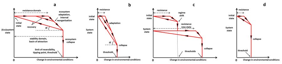
Figure 1. Schematic representation of the trajectories of a (socio-)ecological system in a plane defined by the system state (fundamental structure, processes, and functioning - vertical axis) and the change of environmental conditions (horizontal axis), for different resilience characteristics (a, b, c, d). The initial state corresponds to the position on the graph at the vertical axis (zero change in environmental conditions). In all situations the ecosystem is assumed to collapse irreversibly (down to the horizontal axis) when the change in environmental conditions is much greater than the systems' resistance. The angle
[math]\alpha[/math] represents the rate at which the system recovers when the change in environmental conditions is reduced (small
[math]\alpha[/math] means slow recovery, large
[math]\alpha[/math] means fast recovery). Panel a: Resilience characterized by high resistance (definition 3) and slow recovery (definition 4). Panel b: Resilience characterized by low resistance and fast recovery. Panel c: Resilience characterized by a shift to an alternative stable system state. Panel d: Low resilience, characterized by low resistance and slow recovery.
When considering the potential effect of a certain type of disturbance it is thus useful to ask two questions:
- Will the species of this system be able to tolerate it (implying resistance), and if not,
- Is recovery possible through a successional trajectory, back to the same, or at least a desirable, ecosystem state (implying resilience)?
Resistance breaks down when uni-directional ongoing change acts faster than the organisms' ability to adapt their tolerances. If uni-directional ongoing change is this fast (even if gradual), the system will not be sufficiently resilient either, as full recovery through succession will then not be possible. Recovery from sudden and local disturbance is often possible through recolonization, but the rate of recovery will depend crucially on the spatial extent of disturbance. For example, recovery from anoxia could take 5 to 8 months at the scale of square meters (Rossi et al. 2009[14]), but could take 5 to 8 years at the scale of a whole bay (Diaz & Rosenberg 1995[15]).
According to definition (4), the speed at which an ecosystem returns to its former state following a (minor) disturbance can be considered a measure of resilience. The idea is that a system with a short return time is more resilient than one with a long return time. Such resilience measured as (1 / the return time to a stable equilibrium) has also been called engineering resilience. It has however a long history of use among ecologists (Pimm 1982[16], DeAngelis 1992[17], Vos et al. 2005[18]). Resilience is also used in a way that more closely resembles the definition of resistance. Ecological resilience was defined as the amount of disturbance that an ecosystem could withstand without changing self-organized processes and structures (definition 3).
Resilience of coastal systems largely depends on biodiversity, which is a major requirement for allowing ecosystems to adapt to changing conditions. The human impact on the environment through pollution, fisheries, sediment erosion / deposition and global climate change has brought about much faster change than would occur under natural conditions, putting severe stress on many ecosystems. Without genetic diversity, natural selection cannot occur and if natural selection is limited, adaptation is impossible. Preservation of biodiversity and, more specifically, genetic diversity is therefore of paramount importance for successful adaptation to our rapidly changing environments. However, biodiversity may not always protect ecosystems from major abiotic disturbances (Folke et al. 2004[19]).
Resilience through recolonization
To understand resilience of ecosystems it is essential to understand what drives succession within these ecosystems. Succession determines how, and how fast, communities return to their original state, or perhaps enter a new state. Many aspects of succession can be understood in terms of trade-offs between the ability to be either a good early (re)colonizer, or a good competitor. Succession involves a gradual replacement of colonizer/competitor species according to the degree to which they tolerate, facilitate or inhibit certain environmental conditions and other species (Rossi et al. 2009[14]). The extent to which processes of (re)colonization and succession can take place largely determines the recovery of ecosystems after major disruption and is therefore an essential characteristic of the resilience of ecosystems.
In this context, it is important to consider the spatial component of ecosystem resilience. Diversity of structurally and functionally connected landscapes, rich in resources and species, promotes the flow or movement of individuals, genes, and ecological processes. Below certain thresholds of connectivity the capacity to regain structure and function after perturbation is lost (Holl and Aide, 2011; Rudnick et al., 2012;McIntyre et al., 2014; Rappaport et al., 2015; Ricca et al., 2018). Chambers et al. (2019[20]), based on Allen et al. (2016[21]), have therefore introduced the concept of 'spatial resilience', which is a measure of how spatial attributes, processes, and feedbacks vary over space and time in response to disturbances and affect the resilience of ecosystems. Self-organization through strong feedbacks at multiple scales and high levels of functional diversity and redundancy, stabilizes the system with respect to disturbances within the range of historic variability.
When creating Marine Protected Areas, the sources of populations at all stages of succession should be protected, to preserve 'ecological memory' to the fullest possible extent. This includes protecting not only 'high quality' habitats that harbour healthy mature communities, but also 'low quality' and disturbed habitats that are required for those species that contribute to early recovery of perturbed areas (Rossi et al. 2009[14]). The selection of Marine Protected Areas thus involves evaluating
the number, size, and spatial configuration of habitat fragments and degree of connectivity required to support restoration of ecosystems and conservation of focal habitats and species[20][2].
Resistance to changes in abiotic and biotic factors
Community composition and ecosystem function may change very little under environmental change when the organisms can adapt to such change or tolerate it for some time (when the change is only temporary). However, all organisms have bounds to what they can temporarily or permanently tolerate, and when change exceeds some of these limits, the community composition and ecosystem functioning is likely to change.
It is unlikely that communities can be resistant to ongoing gradual change, such as global warming. Acclimation and phenotypic plasticity do not suffice to maintain the system as it is. Genetic adaptation could allow community members to track such abiotic environmental change, but it is more likely that the area where the community is functioning will be invaded by species that function well at higher temperatures. The original species will thus have to deal with new competitors and predators, in addition to the changed abiotic factor. To some extent the original community can track the preferred temperature range, by moving spatially to greater depths or to alternative geographic areas. But these new areas are likely to differ in other ecological aspects such as water pressure, light climate and perhaps speeds of water flow etc.
Adaptation and the consequences of mortality at different trophic levels
External disturbance interacts with internal mechanisms that shape community structure. To understand how an increased mortality of top-predators will affect the entire food chain, it is essential to understand how processes of mutual adaptation within food chains already give shape to existing patterns such as trophic structure (how biomass in ecosystems is partitioned between trophic levels).
Abundances at different trophic levels (such as algae, herbivores, carnivores and top-predators) and their responses to increased mortality (as under environmental change) depend critically on different mechanisms of adaptation within food chains and on the importance of population density at each of these trophic levels. However, different types of adaptation to living in a food chain context (balancing the need to acquire resources with the need to avoid predation) can often have similar consequences. For example, micro-evolution of behaviour, species replacement and induced defenses at a middle trophic level may all have similar effects on trophic level abundances in disturbed food chains (Abrams and Vos 2003[22]).
Related articles
- Integrated Coastal Zone Management (ICZM)
- Thresholds of environmental sustainablility
- Sustainability indicators
References
- ↑ 1.0 1.1 Lake, P.S. 2013. Resistance, Resilience and Restoration. Ecological Management and Restoration 14: 20-24
- ↑ 2.0 2.1 Olsson, S., Melvin, A. and Giles, S. (eds.) 2019. Climate change and ecosystems. Procs. Sackler Forum on Climate Change and Ecosystems, Washington, DC, November 8-9, 2018, organized by the National Academy of Sciences and The Royal Society
- ↑ Folke, C., Carpenter, S. R., Walker, B., Scheffer, M., Chapin, T. and Rockstrom, J. 2010. Resilience thinking: integrating resilience, adaptability and transformability. Ecology and Society 15(4): 20
- ↑ Scheffer, M. 2009. Critical transitions in nature and society. Princeton University Press, Princeton, New Jersey, USA
- ↑ 5.0 5.1 Brand, F.S. and K. Jax. 2007. Focusing the meaning(s) of resilience: resilience as a descriptive concept and a boundary object. Ecology and Society 12(1):23
- ↑ 6.0 6.1 6.2 Haines‐Young, R. and Potschin. M. (eds.) 2010. The Resilience of Ecosystems to Environmental Change (RECCE). Overview Report, 27 pp. Defra Project Code: NR0134
- ↑ Holling, C.S. 1973. Resilience and stability of ecological systems. Annual Rev. Ecol. Syst. 4: 1–23. doi: 10.1146/annurev.es.04.110173.000245
- ↑ Gunderson, L.H. 2000. Ecological Resilience - in Theory and Application. Annual Review of Ecology and Systematics 31:425-439.
- ↑ Hirota,M., Holmgren,M., Van Nes, E. H, and Scheffer,M. 2011. Global resilience of tropical forest and savanna to critical transitions. Science 334: 232–235. doi: 10.1126/science.1210657
- ↑ Chambers, J. C., Bradley, B. A., Brown, C. S., D’Antonio, C., Germino, M. J., Grace, J. B., et al. 2014. Resilience to stress and disturbance, and resistance to Bromus tectorum L. invasion in the cold desert shrublands of western North America. Ecosystems 7: 360–375. doi: 10.1007/s10021-013-9725-5
- ↑ Pope, K. L., Allen, C. R., and Angeler, D. G. 2014. Fishing for resilience. T. N. Am. Fisheries Soc. 143: 467–478. doi: 10.1080/00028487.2014.880735
- ↑ Seidl, R., Spies, T. A., Peterson, D. L., Stephens, S. L., and Hick, J. A. 2016. Searching for resilience: addressing the impacts of changing disturbance regimes on forest ecosystem services. J. Appl. Ecol. 53 : 120–129. doi: 10.1111/1365-2664.12511
- ↑ 13.0 13.1 Dawson, T.P., Rounsevell, M.D.A., Kluvankova‐Oravska, T., Chobotova V. and Stirling, A. 2010. Dynamic properties of complex adaptive ecosystems: implications for the sustainability of services provision. Biodiversity and Conservation 19: 2843‐2853
- ↑ 14.0 14.1 14.2 Rossi, F., Vos, M. & Middelburg, J.J. 2009. Species identity, diversity and microbial carbon flow in reassembling macrobenthic communities. Oikos 118: 503-512.
- ↑ Diaz, R.J. & Rosenberg, R. 1995. Marine benthic hypoxia: a review of its ecological effects and the behavioural responses of benthic macrofauna. Oceanogr. Mar. Biol. Annu. Rev. 33:245-303.
- ↑ Pimm, S.L. 1982. Food Webs. The University of Chicago Press.
- ↑ DeAngelis, D.L. 1992. Dynamics of Nutrient Cycling and Food Webs. Chapman and Hall, London.
- ↑ Vos, M., Kooi, B.W., DeAngelis, D.L. & Mooij, W.M. 2005. Inducible defenses in food webs. In: Dynamic Food Webs. Multispecies Assemblages, Ecosystem Development and Environmental Change. Eds. P.C. de Ruiter, V. Wolters & J.C. Moore. Academic Press. Pp. 114-127.
- ↑ Folke, C., Carpenter, S., Walker, B., Scheffer, M., Elmqvist, T., Gunderson, L. & Holling, C.S. 2004. Regime Shifts, Resilience, and Biodiversity in Ecosystem Management. Annual Review of Ecolog and Systematics 35:557-581.
- ↑ 20.0 20.1 Chambers, J.C., Allen, C.R. and Cushman, S.A. 2019. Operationalizing Ecological Resilience Concepts for Managing Species and Ecosystems at Risk. Front. Ecol. Evol. 7:241. doi: 10.3389/fevo.2019.00241
- ↑ Allen, C. R., Angeler, D. G., Cumming, G. S., Folk, C., Twidwell, D., and Uden, D. R. 2016. Quantifying spatial resilience. J. Appl. Ecol. 53, 625–635. doi: 10.1111/1365-2664.12634
- ↑ Abrams, P.A & Vos, M. 2003. Adaptation, density dependence and the responses of trophic level abundances to mortality. Evolutionary Ecology Research 5: 1113-1132
