Difference between revisions of "Statistical description of wave parameters"
Dronkers J (talk | contribs) |
Dronkers J (talk | contribs) |
||
| Line 1: | Line 1: | ||
| − | Because of the random nature of natural waves, a statistical description of the waves is normally always used. | + | |
| + | {{Review | ||
| + | |name=Job Dronkers|AuthorID=120| | ||
| + | }} | ||
| + | |||
| + | |||
| + | Because of the random nature of natural waves, a statistical description of the waves is normally always used. Observed wave heights often follow the Rayleigh distribution. Statistical wave parameters are calculated based on this distribution. The most commonly used variables in coastal engineering are described below. | ||
==Most commonly used variables in coastal engineering== | ==Most commonly used variables in coastal engineering== | ||
| + | |||
===Significant wave height=== | ===Significant wave height=== | ||
| − | The significant wave height, | + | |
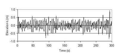
| − | + | [[image:timeseries.jpg|400px|thumb|left|Fig. 1. Time-series of surface elevations by individual waves for a certain sea state.]] | |
| + | |||
| + | An example of a wave record representative for a certain sea state is shown in Fig. 1. The significant wave height, <math>H_s</math>, is the mean of the highest third of the waves; instead of <math>H_s</math> the notation <math>H_{1/3}</math> is also often used. <math>H_s</math> corresponds well with the average height of the highest waves in a wave group. The significant wave height can also be computed from the wave energy; it is then referred to as <math>H_{m0}</math>. In practice it appears that <math>H_{m0} \approx H_s</math>. An explanation, definitions and formulas are given in appendix A. | ||
===Mean wave period=== | ===Mean wave period=== | ||
| − | The mean wave period, | + | The mean wave period, <math>T_m</math>, is the mean of all wave periods in a time-series representing a certain sea state. |
| + | |||
| + | |||
===Peak wave period=== | ===Peak wave period=== | ||
| − | The peak wave period, | + | |
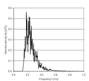
| + | [[image:wavespectrum.jpg|right|thumb|Fig. 2. Wave spectrum: <math>H_{m0}=1m, T_{02}=3.55s, T_p=5s</math> (corresponding to peak frequency of 0.2 <math>s^{-1}</math>)]] | ||
| + | |||
| + | |||
| + | |||
| + | The peak wave period, <math>T_p</math>, is the wave period with the highest energy. The analysis of the distribution of the wave energy as a function of wave frequency <math>f=1/T</math> for a time-series of individual waves is referred to as a spectral analysis. Wind wave periods (frequencies) often follow the so-called JONSWAP or Pierson-Moskowitz spectra (see appendix B). The peak wave period is extracted from the spectra. As a rule of thumb the following relation can be used: | ||
| + | |||
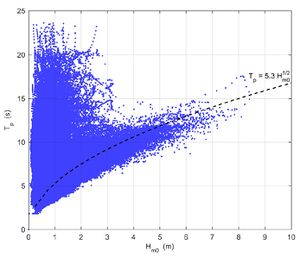
| + | <math>T_p \approx 5 \sqrt{H_{m0}}. \qquad (1) </math> | ||
===Mean wave direction=== | ===Mean wave direction=== | ||
| − | The mean wave direction, | + | The mean wave direction, <math>\theta_m</math>, is defined as the mean of all the individual wave directions in a time-series representing a certain sea state. |
| + | |||
| + | |||
| + | |||
| + | |||
| + | |||
| + | |||
| + | ==Description of wave conditions== | ||
| − | |||
| − | |||
These parameters are often calculated from continuous or periodic time-series of the surface elevations; typically the parameters are calculated once every one or three hours, whereby a new discrete time-series of the statistical wave parameters is constructed. This time-series is thereafter analysed statistically to arrive at a condensed description of the wave conditions as follows: | These parameters are often calculated from continuous or periodic time-series of the surface elevations; typically the parameters are calculated once every one or three hours, whereby a new discrete time-series of the statistical wave parameters is constructed. This time-series is thereafter analysed statistically to arrive at a condensed description of the wave conditions as follows: | ||
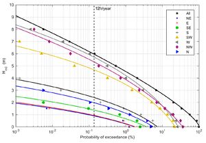
| − | *Wave height distribution represented by | + | *Wave height distribution represented by <math>H_s</math> vs. percentage of exceedance. This often follows a Weibull-distribution (see appendix A and the example in Fig. 3); |
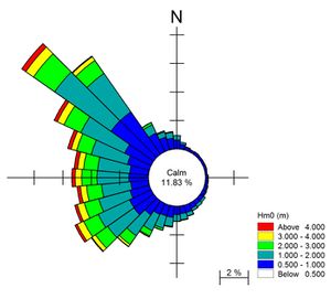
| − | *Directional distribution of the wave heights, which is often presented in the form of a wave rose | + | *Directional distribution of the wave heights, which is often presented in the form of a wave rose (see appendix B and the example in Fig. 4); |
| − | *Scatter diagram of | + | *Scatter diagram of <math>T_p</math> vs. <math>H_s</math> (example in Fig. 5). |
| + | |||
| + | |||
| + | {| border="0" | ||
| + | |- | ||
| + | | valign="top"| | ||
| + | [[File:WaveHeightExceedanceDistribution.jpg|thumb|300px|left|Fig. 3. Wave height exceedance distribution for various wave directions; wave climate from the West Coast of Denmark. ]] | ||
| + | | valign="top"| | ||
| + | [[File:WaveHeightDirectionalSpreading.jpg|thumb|left|300px||Fig. 4. Wave height directional distribution, a so-called wave rose. Wave climate from the West Coast of Denmark.]] | ||
| + | | valign="top"| | ||
| + | [[File:ScatterDiagramWavePeriodWaveHeight.jpg|thumb|left|300px|Fig. 5. Scatter diagram of <math>T_p</math> vs. <math>H_{m0}</math>; wave climate from the West Coast of Denmark. The approximate empirical relation between <math>T_p</math> and <math>H_{m0}</math> for storm waves is also shown. ]] | ||
| + | |} | ||
| + | |||
| + | |||
| + | |||
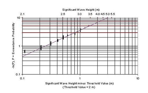
| + | Analyses of extreme wave conditions are performed on the basis of max. wave heights in single storm events or on the basis of annual max. wave heights. These analyses are often presented as exceedence probability vs. wave heights, see Fig. 6 for an example. | ||
| + | |||
| + | [[image:extreme value.jpg|thumb|center|500px|Fig. 6. Extreme value analysis of wave height by Weibull distribution. Threshold = 2 m.]] | ||
| + | |||
| + | |||
| + | |||
| + | |||
| + | ==Further reading== | ||
| + | * Mangor, K., Drønen, N.K., Kaergaard, K.H. and Kristensen, S.E. 2017. Shoreline Management Guidelines. DHI Water and Environment, 451pp. <ref>https://www.dhigroup.com/upload/campaigns/ShorelineManagementGuidelines_Feb2017.pdf</ref> | ||
| + | * Coastal Engineering Manual, part II, chapter 1. US Army Corps of Engineers (USACE), 2008 | ||
| + | |||
| + | |||
| + | |||
| + | ==Appendix A: Rayleigh distribution== | ||
| + | |||
| + | The wave contribution to the ocean sea level <math>\eta(x,y,t)</math> at a certain location <math>x,y</math> is generally a superposition of a large number <math>n</math> of random waves with amplitudes <math>a_j</math>, radial frequencies <math>\omega_j</math> and random phases <math>\phi_j</math>, originating from different nearby and remote regions. This superposition can be represented by | ||
| + | |||
| + | <math>\eta=Re[\sum_{j=1}^{n} a_j \exp(i\omega_j t + i\phi_j)]. \qquad (A1)</math> | ||
| + | |||
| + | The statistical distribution of wave heights was derived by Longuet-Higgins (1952)<ref>Longuet-Higgins, M.S. 1952. On the statistical distribution of sea waves. Journal of Marine Research 11: 245-266</ref> under a few specific conditions: (a) the random numbers <math>a=\sum_{j=1}^{n} a_j \cos\phi_j, \, b=\sum_{j=1}^{n} a_j \sin\phi_j</math> are statistically independent and normally (Gaussian) distributed; (b) the radial frequencies <math>\omega_j</math> of the random waves are grouped in a single narrow band around a central frequency <math>\omega</math> such that <math>|\omega_j -\omega_j'|/ \omega << 1</math> for each <math>j, j'</math>. Under this last condition the expression (A1) may be approximated for the time interval [<math>-\pi / \omega <t< \pi / \omega</math>] by | ||
| + | |||
| + | <math>\eta \approx Re[ \exp(i \omega t) \sum_{j=1}^{n} a_j \exp(i\phi_j)] \equiv \frac{1}{2} H \, Re[\exp(i \omega t+i \phi)] , \quad H = 2 \sqrt{a^2 + b^2} . \qquad (A2)</math> | ||
| + | |||
| + | A well-known mathematical theorem<ref>https://en.wikipedia.org/wiki/Rayleigh_distribution</ref> states that the length of a vector with Gaussian distributed components follows the Rayleigh distribution. In this case the vector length is the wave height <math>H</math> and the components are the random numbers <math>2a, 2b</math>. The Rayleigh probability density function <math>p_R(H)</math> for the wave height <math>H</math> reads: | ||
| + | |||
| + | <math>p_R(H) = \Large\frac{2H}{H_{rms}^2}\normalsize \exp\Large (–(\frac{H}{H_{rms}})^2)\normalsize . \qquad (A3)</math> | ||
| + | |||
| + | The mean square root wave heigth <math>H_{rms}</math> is related to the average wave energy <math>\overline E</math>: | ||
| + | |||
| + | <math> H_{rms}^2 = \int_0^{\infty} p_R(H) H^2 dH =\Large\frac{8}{g \rho}\normalsize \overline E. \qquad (A4)</math> | ||
| + | |||
| + | The average wave height <math>\overline H</math> is related to the mean square root wave height <math>H_{rms}</math> by | ||
| + | |||
| + | <math>\overline H= \int_0^{\infty} p_R(H) H dH = \Large\frac{\sqrt{\pi}}{2}\normalsize H_{rms} | ||
| + | \approx 0.89 H_{rms} .\qquad (A5)</math> | ||
| + | |||
| + | The cumulative Rayleigh distribution (probability of wave height <math><H</math>) is given by | ||
| + | |||
| + | <math>P_R(H)=\int_0^H p_R(H')dH' = 1-\exp\Large (-(\frac{H}{H_{rms}})^2)\normalsize .\qquad (A6) </math> | ||
| + | |||
| + | For calculating <math>H_{1/3}</math> (the mean of the highest third of the waves) we first determine the lowest of the largest third waves, <math>H_l</math>, from the condition <math>P_R(H_l)=2/3</math>, yielding <math>H_l=H_{rms} \ln(3)</math>. The significant wave height <math>H_s \equiv H_{1/3}</math> is given by | ||
| + | |||
| + | <math>H_s=\Large\frac{\int_{H_l}^{\infty} p_R(H)HdH}{\int_{H_l}^{\infty} p_R(H)dH }\normalsize \approx 1.6 \overline H = 1.42 H_{rms}. \qquad (A7)</math> | ||
| + | |||
| + | From (A4), (A5) and (A7) it follows that <math>H_s</math> is related to the average wave energy <math>\overline E</math>: | ||
| + | |||
| + | <math>H_s \approx H_{m0} \equiv 4 \Large \sqrt{ \frac{\overline E}{g \rho}}\normalsize . \qquad(A8)</math> | ||
| + | |||
| + | Extreme wave heights can be derived from the Rayleigh distribution in a similar way. For example, the mean of the 1% highest waves is given by | ||
| + | |||
| + | <math>H_{1/100} \approx 2.36 H_{rms} . \qquad (A9)</math> | ||
| + | |||
| + | In spite of the restrictive conditions for which the Rayleigh distribution has been derived, it appears that in many cases it corresponds reasonably well with wave height statistics obtained from field observations, even if the conditions (a) and (b) are not well satisfied. | ||
| + | |||
| + | However, the Rayleigh distribution does not put a limit on the wave height, which is physically unrealistic and leads to overestimation of the highest waves. Therefore often the Weibull distribution is used instead of the Rayleigh distribution. The Weibull distribution <ref>https://en.wikipedia.org/wiki/Weibull_distribution</ref> reads: | ||
| + | |||
| + | <math>p_W(H)=\Large\frac{m}{\lambda}(\frac{H}{\lambda})^{(m-1)}\normalsize \exp\Large (–(\frac{H}{\lambda})^{m}) \normalsize . \qquad (A10)</math> | ||
| + | |||
| + | The Rayleigh distribution corresponds to the Weibull distribution for <math>m=2, \; \lambda=H_{rms}</math>. The Weibull distribution has an additional parameter (<math>m</math>) that allows suppression of the highest waves for <math>m>2</math> and an optimum adjustment to the observed wave data. | ||
| + | |||
| + | This is especially relevant for shallow-water waves, which are truncated due to depth-induced wave breaking. For this situation, alternative distributions have been proposed, for example by Battjes and Groenendijk (2000)<ref> Battjes, J.A. and Groenendijk, H.W. 2000. Wave height distributions on shallow foreshores. Coastal Engineering 40: 161-182</ref>. According to this study, a Weibull distribution with <math>m=3.6</math> should be used above a certain threshold, <math>H_{tr}</math>. | ||
| + | |||
| + | ==Appendix B: Frequency spectrum== | ||
| + | |||
| + | A wave record can further be characterized by its frequency spectrum. The energy density spectrum of a sea state is generally designated by <math>E(f)</math>. The total energy is given by | ||
| + | |||
| + | <math>\overline E=\int_0^{\infty} E(f)df . \qquad (B1)</math> | ||
| + | |||
| + | The wave frequency spectrum can be determined from a wave record by using a Fourier transform. It can also be determined by modelling the wind-induced wave field in a large source area. Empirical formulas have been established for fully developed wave fields under constant wind stress. For deep water without fetch restriction, it is recommended to use the adapted Pierson-Moskowitz frequency distribution <math>E_{PM}</math> <ref>The Rock Manual. The use of rock in hydraulic engineering (2nd edition).CIRIA. London, 2007</ref>: | ||
| + | |||
| + | <math>E_{PM}(f)=3.26 \Large\frac{\overline E}{f_p}(\frac{f_p}{f})^4 e^{-(\frac{f_p}{f})^4}\normalsize . \qquad (B2)</math> | ||
| + | |||
| + | For the average wave energy <math>\overline E</math> and the peak frequency <math>f_p</math> the following empirical expressions are found: | ||
| + | |||
| + | <math>\overline E \approx 0.005 \rho g^{-1} U_{10}^4\; , \; f_p \approx 0.123 g U_{10}^{-1} \;,</math> | ||
| + | where <math>g</math> is the gravitational acceleration and <math>U_{10}</math> the wind velocity at 10 m above the sea surface. | ||
| − | + | For fetch-limited seas, the spectrum is more strongly peaked around the peak frequency. For this situation, the empirical JONSWAP spectrum can be used. It has the form | |
| − | + | <math>E_{WONSJAP}=\Large\frac{\alpha \rho g^3}{f_p (2 \pi f_p)^4} (\frac{f_p}{f})^4 e^{-(\frac{f_p}{f})^4}\normalsize \gamma^\delta \;, \quad \delta =e^{-\Large\frac{1}{2}\Large(\frac{(f/f_p)-1}{\sigma})^2}\normalsize , \qquad (B3)</math>, | |
| − | + | where the parameters <math>\alpha, \gamma, \sigma, f_p</math> depend on the fetch length and should be fitted to the wave data. For <math>\gamma=1</math> the Pierson-Moskowitz and JONSWAP spectra are the same. | |
| − | |||
| − | |||
| − | |||
| − | |||
| − | < | + | Different characteristic wave periods can be derived from the wave spectrum: the significant wave period <math>T_{01}</math>, the mean wave period <math>T_{02}</math> and the mean energy period <math>T_E</math>. They are given by the expressions |
| + | <math>T_{01}=\Large\frac{\int_0^{\infty} E(f)df}{\int_0^{\infty} E(f)fdf }\normalsize, \quad T_{02}=\Large \sqrt{\frac{\int_0^{\infty} E(f)df}{\int_0^{\infty} E(f) f^2 df }}\normalsize, \quad T_E=\Large\frac{\int_0^{\infty} E(f) f^{-1} df}{\int_0^{\infty} E(f)df }\normalsize \; .\qquad (B4) </math> | ||
| + | |||
| + | For the Pierson-Moskowitz distribution (B2) we have | ||
| + | |||
| + | <math>T_{01}=0.69 \, T_p, \; T_{02}=0.58 \, T_p, \; T_E=0.82 \, T_p </math>. | ||
| + | |||
| + | A closer estimate of the peak period <math>T_p=1/f_p</math> can be obtained by using a higher power of the energy density spectrum, for example | ||
| + | |||
| + | <math>\Large\frac{\int_0^{\infty} E^5(f)df}{\int_0^{\infty} E^5(f)fdf }\normalsize \approx 0.95 T_p</math>. | ||
| + | |||
| + | In the fetch-limited case with a JONSWAP-type spectrum the value of <math>T_E</math> is generally found close to the peak period <math>T_p</math>. | ||
| + | |||
| + | |||
| + | In an irregular wave field, waves may come from different directions. The wave incidence direction is an important parameter for sediment transport in the coastal zone. Waves originating from different areas may have different spectra. The directional spread of incoming waves for a particular wave frequency can be represented by a distribution function <math>D(f,\theta)</math>, where <math>\theta</math> is the wave incidence angle. We then have | ||
| + | |||
| + | <math>\overline E \equiv \int_0^{\infty} \int_0^{2 \pi} S(f, \theta) df d \theta \equiv \int_0^{\infty} \int_0^{2 \pi} E(f) \, D(f, \theta) df d \theta \; ,\quad \int_0^{2 \pi} D(f, \theta) d \theta =1 \; .\qquad (B5) </math> | ||
| + | |||
| + | The directional wave spectrum <math>S(f, \theta)</math> can be derived from directional wave buoys. In practice, it is often obtained by numerical modelling of the wave field in the major source area. | ||
| + | |||
| + | |||
| + | |||
==References== | ==References== | ||
<references/> | <references/> | ||
| − | |||
| − | |||
| − | |||
Revision as of 17:27, 15 December 2019
Because of the random nature of natural waves, a statistical description of the waves is normally always used. Observed wave heights often follow the Rayleigh distribution. Statistical wave parameters are calculated based on this distribution. The most commonly used variables in coastal engineering are described below.
Contents
Most commonly used variables in coastal engineering
Significant wave height
An example of a wave record representative for a certain sea state is shown in Fig. 1. The significant wave height, [math]H_s[/math], is the mean of the highest third of the waves; instead of [math]H_s[/math] the notation [math]H_{1/3}[/math] is also often used. [math]H_s[/math] corresponds well with the average height of the highest waves in a wave group. The significant wave height can also be computed from the wave energy; it is then referred to as [math]H_{m0}[/math]. In practice it appears that [math]H_{m0} \approx H_s[/math]. An explanation, definitions and formulas are given in appendix A.
Mean wave period
The mean wave period, [math]T_m[/math], is the mean of all wave periods in a time-series representing a certain sea state.
Peak wave period
The peak wave period, [math]T_p[/math], is the wave period with the highest energy. The analysis of the distribution of the wave energy as a function of wave frequency [math]f=1/T[/math] for a time-series of individual waves is referred to as a spectral analysis. Wind wave periods (frequencies) often follow the so-called JONSWAP or Pierson-Moskowitz spectra (see appendix B). The peak wave period is extracted from the spectra. As a rule of thumb the following relation can be used:
[math]T_p \approx 5 \sqrt{H_{m0}}. \qquad (1) [/math]
Mean wave direction
The mean wave direction, [math]\theta_m[/math], is defined as the mean of all the individual wave directions in a time-series representing a certain sea state.
Description of wave conditions
These parameters are often calculated from continuous or periodic time-series of the surface elevations; typically the parameters are calculated once every one or three hours, whereby a new discrete time-series of the statistical wave parameters is constructed. This time-series is thereafter analysed statistically to arrive at a condensed description of the wave conditions as follows:
- Wave height distribution represented by [math]H_s[/math] vs. percentage of exceedance. This often follows a Weibull-distribution (see appendix A and the example in Fig. 3);
- Directional distribution of the wave heights, which is often presented in the form of a wave rose (see appendix B and the example in Fig. 4);
- Scatter diagram of [math]T_p[/math] vs. [math]H_s[/math] (example in Fig. 5).
Analyses of extreme wave conditions are performed on the basis of max. wave heights in single storm events or on the basis of annual max. wave heights. These analyses are often presented as exceedence probability vs. wave heights, see Fig. 6 for an example.
Further reading
- Mangor, K., Drønen, N.K., Kaergaard, K.H. and Kristensen, S.E. 2017. Shoreline Management Guidelines. DHI Water and Environment, 451pp. [1]
- Coastal Engineering Manual, part II, chapter 1. US Army Corps of Engineers (USACE), 2008
Appendix A: Rayleigh distribution
The wave contribution to the ocean sea level [math]\eta(x,y,t)[/math] at a certain location [math]x,y[/math] is generally a superposition of a large number [math]n[/math] of random waves with amplitudes [math]a_j[/math], radial frequencies [math]\omega_j[/math] and random phases [math]\phi_j[/math], originating from different nearby and remote regions. This superposition can be represented by
[math]\eta=Re[\sum_{j=1}^{n} a_j \exp(i\omega_j t + i\phi_j)]. \qquad (A1)[/math]
The statistical distribution of wave heights was derived by Longuet-Higgins (1952)[2] under a few specific conditions: (a) the random numbers [math]a=\sum_{j=1}^{n} a_j \cos\phi_j, \, b=\sum_{j=1}^{n} a_j \sin\phi_j[/math] are statistically independent and normally (Gaussian) distributed; (b) the radial frequencies [math]\omega_j[/math] of the random waves are grouped in a single narrow band around a central frequency [math]\omega[/math] such that [math]|\omega_j -\omega_j'|/ \omega \lt \lt 1[/math] for each [math]j, j'[/math]. Under this last condition the expression (A1) may be approximated for the time interval [[math]-\pi / \omega \lt t\lt \pi / \omega[/math]] by
[math]\eta \approx Re[ \exp(i \omega t) \sum_{j=1}^{n} a_j \exp(i\phi_j)] \equiv \frac{1}{2} H \, Re[\exp(i \omega t+i \phi)] , \quad H = 2 \sqrt{a^2 + b^2} . \qquad (A2)[/math]
A well-known mathematical theorem[3] states that the length of a vector with Gaussian distributed components follows the Rayleigh distribution. In this case the vector length is the wave height [math]H[/math] and the components are the random numbers [math]2a, 2b[/math]. The Rayleigh probability density function [math]p_R(H)[/math] for the wave height [math]H[/math] reads:
[math]p_R(H) = \Large\frac{2H}{H_{rms}^2}\normalsize \exp\Large (–(\frac{H}{H_{rms}})^2)\normalsize . \qquad (A3)[/math]
The mean square root wave heigth [math]H_{rms}[/math] is related to the average wave energy [math]\overline E[/math]:
[math] H_{rms}^2 = \int_0^{\infty} p_R(H) H^2 dH =\Large\frac{8}{g \rho}\normalsize \overline E. \qquad (A4)[/math]
The average wave height [math]\overline H[/math] is related to the mean square root wave height [math]H_{rms}[/math] by
[math]\overline H= \int_0^{\infty} p_R(H) H dH = \Large\frac{\sqrt{\pi}}{2}\normalsize H_{rms} \approx 0.89 H_{rms} .\qquad (A5)[/math]
The cumulative Rayleigh distribution (probability of wave height [math]\lt H[/math]) is given by
[math]P_R(H)=\int_0^H p_R(H')dH' = 1-\exp\Large (-(\frac{H}{H_{rms}})^2)\normalsize .\qquad (A6) [/math]
For calculating [math]H_{1/3}[/math] (the mean of the highest third of the waves) we first determine the lowest of the largest third waves, [math]H_l[/math], from the condition [math]P_R(H_l)=2/3[/math], yielding [math]H_l=H_{rms} \ln(3)[/math]. The significant wave height [math]H_s \equiv H_{1/3}[/math] is given by
[math]H_s=\Large\frac{\int_{H_l}^{\infty} p_R(H)HdH}{\int_{H_l}^{\infty} p_R(H)dH }\normalsize \approx 1.6 \overline H = 1.42 H_{rms}. \qquad (A7)[/math]
From (A4), (A5) and (A7) it follows that [math]H_s[/math] is related to the average wave energy [math]\overline E[/math]:
[math]H_s \approx H_{m0} \equiv 4 \Large \sqrt{ \frac{\overline E}{g \rho}}\normalsize . \qquad(A8)[/math]
Extreme wave heights can be derived from the Rayleigh distribution in a similar way. For example, the mean of the 1% highest waves is given by
[math]H_{1/100} \approx 2.36 H_{rms} . \qquad (A9)[/math]
In spite of the restrictive conditions for which the Rayleigh distribution has been derived, it appears that in many cases it corresponds reasonably well with wave height statistics obtained from field observations, even if the conditions (a) and (b) are not well satisfied.
However, the Rayleigh distribution does not put a limit on the wave height, which is physically unrealistic and leads to overestimation of the highest waves. Therefore often the Weibull distribution is used instead of the Rayleigh distribution. The Weibull distribution [4] reads:
[math]p_W(H)=\Large\frac{m}{\lambda}(\frac{H}{\lambda})^{(m-1)}\normalsize \exp\Large (–(\frac{H}{\lambda})^{m}) \normalsize . \qquad (A10)[/math]
The Rayleigh distribution corresponds to the Weibull distribution for [math]m=2, \; \lambda=H_{rms}[/math]. The Weibull distribution has an additional parameter ([math]m[/math]) that allows suppression of the highest waves for [math]m\gt 2[/math] and an optimum adjustment to the observed wave data.
This is especially relevant for shallow-water waves, which are truncated due to depth-induced wave breaking. For this situation, alternative distributions have been proposed, for example by Battjes and Groenendijk (2000)[5]. According to this study, a Weibull distribution with [math]m=3.6[/math] should be used above a certain threshold, [math]H_{tr}[/math].
Appendix B: Frequency spectrum
A wave record can further be characterized by its frequency spectrum. The energy density spectrum of a sea state is generally designated by [math]E(f)[/math]. The total energy is given by
[math]\overline E=\int_0^{\infty} E(f)df . \qquad (B1)[/math]
The wave frequency spectrum can be determined from a wave record by using a Fourier transform. It can also be determined by modelling the wind-induced wave field in a large source area. Empirical formulas have been established for fully developed wave fields under constant wind stress. For deep water without fetch restriction, it is recommended to use the adapted Pierson-Moskowitz frequency distribution [math]E_{PM}[/math] [6]:
[math]E_{PM}(f)=3.26 \Large\frac{\overline E}{f_p}(\frac{f_p}{f})^4 e^{-(\frac{f_p}{f})^4}\normalsize . \qquad (B2)[/math]
For the average wave energy [math]\overline E[/math] and the peak frequency [math]f_p[/math] the following empirical expressions are found:
[math]\overline E \approx 0.005 \rho g^{-1} U_{10}^4\; , \; f_p \approx 0.123 g U_{10}^{-1} \;,[/math]
where [math]g[/math] is the gravitational acceleration and [math]U_{10}[/math] the wind velocity at 10 m above the sea surface.
For fetch-limited seas, the spectrum is more strongly peaked around the peak frequency. For this situation, the empirical JONSWAP spectrum can be used. It has the form
[math]E_{WONSJAP}=\Large\frac{\alpha \rho g^3}{f_p (2 \pi f_p)^4} (\frac{f_p}{f})^4 e^{-(\frac{f_p}{f})^4}\normalsize \gamma^\delta \;, \quad \delta =e^{-\Large\frac{1}{2}\Large(\frac{(f/f_p)-1}{\sigma})^2}\normalsize , \qquad (B3)[/math],
where the parameters [math]\alpha, \gamma, \sigma, f_p[/math] depend on the fetch length and should be fitted to the wave data. For [math]\gamma=1[/math] the Pierson-Moskowitz and JONSWAP spectra are the same.
Different characteristic wave periods can be derived from the wave spectrum: the significant wave period [math]T_{01}[/math], the mean wave period [math]T_{02}[/math] and the mean energy period [math]T_E[/math]. They are given by the expressions
[math]T_{01}=\Large\frac{\int_0^{\infty} E(f)df}{\int_0^{\infty} E(f)fdf }\normalsize, \quad T_{02}=\Large \sqrt{\frac{\int_0^{\infty} E(f)df}{\int_0^{\infty} E(f) f^2 df }}\normalsize, \quad T_E=\Large\frac{\int_0^{\infty} E(f) f^{-1} df}{\int_0^{\infty} E(f)df }\normalsize \; .\qquad (B4) [/math]
For the Pierson-Moskowitz distribution (B2) we have
[math]T_{01}=0.69 \, T_p, \; T_{02}=0.58 \, T_p, \; T_E=0.82 \, T_p [/math].
A closer estimate of the peak period [math]T_p=1/f_p[/math] can be obtained by using a higher power of the energy density spectrum, for example
[math]\Large\frac{\int_0^{\infty} E^5(f)df}{\int_0^{\infty} E^5(f)fdf }\normalsize \approx 0.95 T_p[/math].
In the fetch-limited case with a JONSWAP-type spectrum the value of [math]T_E[/math] is generally found close to the peak period [math]T_p[/math].
In an irregular wave field, waves may come from different directions. The wave incidence direction is an important parameter for sediment transport in the coastal zone. Waves originating from different areas may have different spectra. The directional spread of incoming waves for a particular wave frequency can be represented by a distribution function [math]D(f,\theta)[/math], where [math]\theta[/math] is the wave incidence angle. We then have
[math]\overline E \equiv \int_0^{\infty} \int_0^{2 \pi} S(f, \theta) df d \theta \equiv \int_0^{\infty} \int_0^{2 \pi} E(f) \, D(f, \theta) df d \theta \; ,\quad \int_0^{2 \pi} D(f, \theta) d \theta =1 \; .\qquad (B5) [/math]
The directional wave spectrum [math]S(f, \theta)[/math] can be derived from directional wave buoys. In practice, it is often obtained by numerical modelling of the wave field in the major source area.
References
- ↑ https://www.dhigroup.com/upload/campaigns/ShorelineManagementGuidelines_Feb2017.pdf
- ↑ Longuet-Higgins, M.S. 1952. On the statistical distribution of sea waves. Journal of Marine Research 11: 245-266
- ↑ https://en.wikipedia.org/wiki/Rayleigh_distribution
- ↑ https://en.wikipedia.org/wiki/Weibull_distribution
- ↑ Battjes, J.A. and Groenendijk, H.W. 2000. Wave height distributions on shallow foreshores. Coastal Engineering 40: 161-182
- ↑ The Rock Manual. The use of rock in hydraulic engineering (2nd edition).CIRIA. London, 2007
Please note that others may also have edited the contents of this article.
|
