Difference between revisions of "Statistical description of wave parameters"
Dronkers J (talk | contribs) |
|||
| (44 intermediate revisions by 3 users not shown) | |||
| Line 1: | Line 1: | ||
| − | |||
| + | Because of the random nature of natural waves, a statistical description is normally always used. A fair approximation of the observed distribution of wave heights is given by the Rayleigh distribution. Statistical wave parameters are often calculated based on this distribution. The most commonly used variables in coastal engineering are described below. | ||
| + | |||
| + | ==Most commonly used variables in coastal engineering== | ||
| + | |||
| + | ===Significant wave height=== | ||
| + | |||
| + | [[image:timeseries.jpg|400px|thumb|left|Fig. 1. Time-series of surface elevations by individual waves for a certain sea state.]] | ||
| + | |||
| + | An example of a wave record representative for a certain sea state is shown in Fig. 1. The ''significant wave height'', <math>H_s</math>, is the mean of the highest third of the waves; instead of <math>H_s</math> the notation <math>H_{1/3}</math> is also often used. <math>H_s</math> represents well the average height of the highest waves in a wave group. The significant wave height can also be computed from the wave energy. For non-breaking waves it appears that <math>H_s \approx H_{m0} = 4 [<E> / (g \rho)]^{1/2}, </math> where <math>H_{m0}</math> is the ''spectral significant wave height''. An explanation, definitions and formulas are given in appendix A. | ||
| + | |||
| + | ===Mean wave period=== | ||
| + | The mean wave period, <math>T_m</math>, is the mean of all wave periods in a time-series representing a certain sea state. | ||
| + | |||
| + | |||
| + | |||
| + | ===Peak wave period=== | ||
| + | |||
| + | [[image:wavespectrum.jpg|right|thumb|Fig. 2. Wave spectrum: <math>H_{m0}=1m, T_{02}=3.55s, T_p=5s</math> (corresponding to peak frequency of 0.2 <math>s^{-1}</math>)]] | ||
| + | |||
| + | |||
| + | |||
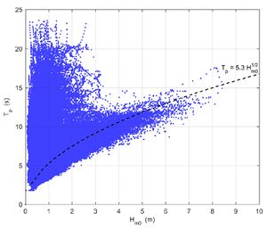
| + | The peak wave period, <math>T_p</math>, is the wave period with the highest energy. The analysis of the distribution of the wave energy as a function of wave frequency <math>f=1/T</math> for a time-series of individual waves is referred to as a spectral analysis. Wind wave periods (frequencies) often follow the so-called JONSWAP or Pierson-Moskowitz spectra (see appendix B). The peak wave period is extracted from the spectra. As a rule of thumb the following relation can be used, see Fig. 5<ref> Mangor, K., Drønen, N.K., Kaergaard, K.H. and Kristensen, S.E. 2017. Shoreline Management Guidelines. DHI Water and Environment, 451pp.</ref>: | ||
| + | |||
| + | <math>T_p \approx 5 \sqrt{H_{m0}}. \qquad (1) </math> | ||
| + | |||
| + | ===Mean wave direction=== | ||
| + | The mean wave direction, <math>\theta_m</math>, is defined as the mean of all the individual wave directions in a time-series representing a certain sea state. | ||
| + | |||
| + | |||
| + | |||
| + | |||
| + | |||
| + | |||
| + | ==Description of wave conditions== | ||
| + | |||
| + | These various wave parameters are often calculated from continuous or periodic time-series of the surface elevations; typically the parameters are calculated once every one or three hours, whereby a new discrete time-series of the statistical wave parameters is constructed. This time-series is thereafter analyzed statistically to arrive at a condensed description of the wave conditions as follows: | ||
| + | |||
| + | *Wave height distribution represented by <math>H_s</math> vs. percentage of exceedance. This often follows a Weibull-distribution (see appendix A and the example in Fig. 3); | ||
| + | *Directional distribution of the wave heights, which is often presented in the form of a wave rose (see appendix B and the example in Fig. 4); | ||
| + | *Scatter diagram of <math>T_p</math> vs. <math>H_s</math> (example in Fig. 5). | ||
| + | |||
| + | |||
| + | {| border="0" | ||
| + | |- | ||
| + | | valign="top"| | ||
| + | [[File:WaveHeightExceedanceDistribution.jpg|thumb|300px|left|Fig. 3. Wave height exceedance distribution for various wave directions; wave climate from the West Coast of Denmark. ]] | ||
| + | | valign="top"| | ||
| + | [[File:WaveHeightDirectionalSpreading.jpg|thumb|left|300px||Fig. 4. Wave height directional distribution, a so-called wave rose. Wave climate from the West Coast of Denmark.]] | ||
| + | | valign="top"| | ||
| + | [[File:ScatterDiagramWavePeriodWaveHeight.jpg|thumb|left|300px|Fig. 5. Scatter diagram of <math>T_p</math> vs. <math>H_{m0}</math>; wave climate from the West Coast of Denmark. The approximate empirical relation between <math>T_p</math> and <math>H_{m0}</math> for storm waves is also shown. ]] | ||
| + | |} | ||
| + | |||
| + | |||
| + | |||
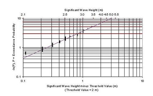
| + | Analyses of extreme wave conditions are performed on the basis of max. wave heights in single storm events or on the basis of annual max. wave heights. These analyses are often presented as exceedance probability vs. wave heights, see Fig. 6 for an example. | ||
| + | |||
| + | [[image:extreme value.jpg|thumb|center|500px|Fig. 6. Extreme value analysis of wave height by Weibull distribution. Threshold = 2 m.]] | ||
| + | |||
| + | |||
| + | |||
| + | |||
| + | ==Further reading== | ||
| + | * Mangor, K., Drønen, N.K., Kaergaard, K.H. and Kristensen, S.E. 2017. Shoreline Management Guidelines. DHI Water and Environment, 451pp. <ref>https://www.dhigroup.com/upload/campaigns/ShorelineManagementGuidelines_Feb2017.pdf</ref> | ||
| + | * Coastal Engineering Manual, part II, chapter 1. US Army Corps of Engineers (USACE), 2008 | ||
| + | |||
| + | |||
| + | |||
| + | ==Appendix A: Rayleigh distribution== | ||
| + | |||
| + | We consider a wave field <math>\eta(x,y,t)</math> consisting of a superposition of <math>n</math> independent, uncorrelated sinusoidal (i.e. linear) waves, with amplitudes <math>a_j</math>, radial frequencies <math>\omega_j</math> and random phases <math>\phi_j</math>, originating from different nearby and remote regions. This superposition can be represented by | ||
| + | |||
| + | <math>\eta=Re[\sum_{j=1}^{n} a_j \exp(i\omega_j t + i\phi_j)]. \qquad (A1)</math> | ||
| + | |||
| + | The statistical distribution of wave heights was derived by Longuet-Higgins (1952)<ref>Longuet-Higgins, M.S. 1952. On the statistical distribution of sea waves. Journal of Marine Research 11: 245-266</ref> under a few specific conditions: (a) the radial frequencies <math>\omega_j</math> of the random waves are grouped in a single narrow band around a central frequency <math>\omega</math> such that <math>|\omega_j -\omega_j'|/ \omega << 1</math> for each <math>j, j' \, ; \;</math> (b) the slowly varying numbers <math>\; a=\sum_{j=1}^{n} a_j \cos \big( \phi_j + (\omega_j - \omega)t \big), \, b=\sum_{j=1}^{n} a_j \sin\big( \phi_j + (\omega_j - \omega)t \big) \;</math> are statistically independent and normally (Gaussian) distributed. Under these conditions the expression (A1) can be approximated for the time interval [<math>-\pi / \omega <t< \pi / \omega</math>] by | ||
| + | |||
| + | <math>\eta \approx \frac{1}{2} H \, \cos(\omega t+ \phi) , \quad H = 2 \sqrt{a^2 + b^2} , \quad \phi = \tan^{-1} (b/a) . \qquad (A2)</math> | ||
| + | |||
| + | A well-known mathematical theorem<ref>https://en.wikipedia.org/wiki/Rayleigh_distribution</ref> states that the length of a vector with Gaussian distributed components follows the Rayleigh distribution. In this case the vector length is the wave height <math>H</math> and the components are the random numbers <math>\sqrt{2}a, \sqrt{2}b</math>. The Rayleigh probability density function <math>p_R(H)</math> for the wave height <math>H</math> reads: | ||
| + | |||
| + | <math>p_R(H) = \Large\frac{2H}{H_{rms}^2}\normalsize \exp\Large (–(\frac{H}{H_{rms}})^2)\normalsize . \qquad (A3)</math> | ||
| + | |||
| + | The root mean square wave height (also called mean energy wave height) <math>H_{rms}</math> is related to the average wave energy <math>< E></math>: | ||
| + | |||
| + | <math> H_{rms}^2 = \int_0^{\infty} p_R(H) H^2 dH =\Large\frac{8}{g \rho}\normalsize < E>. \qquad (A4)</math> | ||
| + | |||
| + | The average wave energy is defined as <math><E> = g \rho \, m_0 \equiv g \rho <(\, \eta(t)-<\eta>)^2></math>, where <math>g</math> is the gravitational acceleration, <math>\rho</math> the seawater density and where <math>\; <…> \; </math> designates the average over a period much longer than the characteristic wave periods. Not considering wave set-up / set-down implies <math><\eta>=0</math>. | ||
| + | |||
| + | The average wave height <math>< H></math> is related to the root mean square wave height <math>H_{rms}</math> by | ||
| + | |||
| + | <math><H>= \int_0^{\infty} p_R(H) H dH = \Large\frac{\sqrt{\pi}}{2}\normalsize H_{rms} | ||
| + | \approx 0.89 H_{rms} .\qquad (A5)</math> | ||
| + | |||
| + | The cumulative Rayleigh distribution (probability of wave height <math><H</math>) is given by | ||
| + | |||
| + | <math>P_R(H)=\int_0^H p_R(H')dH' = 1-\exp\Large (-(\frac{H}{H_{rms}})^2)\normalsize .\qquad (A6) </math> | ||
| + | |||
| + | Assuming that wave heights are Reynolds distributed, relations can be derived between different wave parameters that are often used in practice. For the derivation of the significant wave height <math>H_s \equiv H_{1/3}</math> (the mean of the highest 1/3-part of the waves) we first determine the lowest height of the highest 1/3-part of the waves, <math>H_3</math>, from the condition <math>P_R(H_3)=2/3</math>, yielding <math>H_3=H_{rms} \sqrt{\ln(3)}</math>. The significant wave height is then related to the root mean square wave height by | ||
| + | |||
| + | <math>H_s=\Large\frac{\int_{H_3}^{\infty} p_R(H)HdH}{\int_{H_3}^{\infty} p_R(H)dH }\normalsize = 3 \, \int_{H_3}^{\infty} p_R(H)HdH \approx 1.6 <H> = 1.42 H_{rms}. \qquad (A7)</math> | ||
| + | |||
| + | From Eqs. (A4) and (A7), it follows that the significant wave height <math>H_s</math> is related to the average wave energy <math><E></math> by | ||
| + | |||
| + | <math>H_s \approx H_{m0} \equiv 4 \Large \sqrt{ \frac{<E>}{g \rho}}\normalsize \equiv 4 \sqrt{m_0}. \qquad(A8)</math> | ||
| + | |||
| + | Extreme wave heights can be derived from the Rayleigh distribution in a similar way. For example, the mean of the 1% highest waves is given by | ||
| + | |||
| + | <math>H_{1/100} \approx 1.52 H_s . \qquad (A9)</math> | ||
| + | |||
| + | The Rayleigh distribution has been derived under the rather restrictive conditions ((a) and (b)). Since the Rayleigh distribution does not put a limit on the wave height, it allows for unrealistic high waves. When compared with wave height statistics obtained from field observations, it appears that the Rayleigh distribution tends to overestimate wave heights. This overestimation is greatest (more than 8%) for high long-period waves. Overestimation of the wave height is mainly due to wave breaking, which is related to increasing sharpness of wave peaks in deep water or to depth-induced wave breaking in shallow water<ref>Karmpadakis, I. and Swan, C. 2022. A new crest height distribution for nonlinear and breaking waves in varying water depths. Ocean Engineering 266, 112972</ref>. A broad-banded instead of a narrow-banded wave spectrum can be another reason for wave height overestimation by the Rayleigh distribution<ref>Karmpadakis, I., Swan, C. and Christou, M. 2022. A new wave height distribution for intermediate and shallow water depths. Coastal Engineering 175, 104130</ref>. Unlike wave height, wave crest height is generally underestimated by the Rayleigh distribution. The main reason for underestimating the wave crest height is the neglect of nonlinearity in the wave field<ref>Tayfun, M.A. 1980. Narrow-Band Nonlinear Sea Waves. J. Geophysical Research 85(C3): 1548-1552</ref>. Nonlinearity generates so-called 'skewed' waves: the wave shape changes from sinusoidal to more peaked with narrow wave crests and more shallow and wide wave troughs<ref name=LH>Longuet-Higgins, M.S. 1963. The effect of non-linearities on statistical distributions in the theory of sea waves. J. Fluid Mech. 17: 459-480</ref>. The conditions underlying the Rayleigh distribution are not satisfied in the case of significant nonlinearity, because the wave components in Eq. A1 are not random but correlated to generate a systematic deviation from the sinusoidal shape<ref>Casas‐Prat, M. and Holthuijsen, L. H. 2010. Short‐term statistics of waves observed in deep water. J. Geophys. Res. 115, C09024</ref><ref>Karmpadakis, I., Swan, C. and Christou, M., 2020. Assessment of wave height distributions using an extensive field database. Coastal Engineering 157, 103630</ref>, see Appendix C: Distribution of nonlinear waves. | ||
| + | |||
| + | The Weibull distribution is one of the proposed alternatives to the Rayleigh distribution. The Weibull distribution reads <ref>https://en.wikipedia.org/wiki/Weibull_distribution</ref> : | ||
| + | |||
| + | <math>p_W(H)=\Large\frac{m}{\lambda}(\frac{H}{\lambda})^{(m-1)}\normalsize \exp\Large (–(\frac{H}{\lambda})^{m}) \normalsize . \qquad (A10)</math> | ||
| + | |||
| + | The Rayleigh distribution corresponds to the Weibull distribution for <math>m=2, \; \lambda=H_{rms}</math>. The Weibull distribution has an additional parameter (<math>m</math>) that allows suppression of the highest waves for <math>m>2</math> and an optimum adjustment to the observed wave data. | ||
| + | |||
| + | This is especially relevant for shallow-water waves, which are truncated due to depth-induced wave breaking (see [[Breaker index]]). Because of this truncation, the random numbers <math>a</math> and <math>b</math> in Eq. (2) are not Gaussian distributed; the wave height therefore does not follow a Rayleigh distribution. For this situation, alternative distributions have been proposed, for example by Battjes and Groenendijk (2000)<ref name=BG> Battjes, J.A. and Groenendijk, H.W. 2000. Wave height distributions on shallow foreshores. Coastal Engineering 40: 161-182</ref>. According to this study, a Weibull distribution with <math>m=3.6</math> should be used above a certain threshold, <math>H_{tr}</math> (threshold for depth-induced wave breaking). This implies that the relationships (A7-A9) are not valid in shallow water. For example, if <math>H_{tr}<H_s</math> (i.e. very shallow water), Eq. (A9) should be replaced by <ref name=BG></ref> | ||
| + | |||
| + | <math>H_{1/100} \approx 1.28 H_s . \qquad (A11)</math> | ||
| + | |||
| + | Flume experiments of shallow-water wave transformation show that the value of <math>m</math> is not constant but varies over the surf zone slope (gradual increase followed by decrease<ref>Xu, J., Liu, S., Li, J. and Jia, W. 2021. Experimental study of wave height, crest, and trough distributions of directional irregular waves on a slope. Ocean Engineering 242: 110136</ref>). | ||
| + | |||
| + | ==Appendix B: Frequency spectrum== | ||
| + | |||
| + | A wave record can further be characterized by its frequency spectrum. The energy density spectrum of a sea state is generally designated by <math>E(f)</math>. The total energy is given by | ||
| + | |||
| + | <math><E> =\int_0^{\infty} E(f)df . \qquad (B1)</math> | ||
| + | |||
| + | The wave frequency spectrum can be determined from a wave record <math>\eta(t)</math> by using a Fourier transform as follows: The wave energy averaged over a period <math>[-T/2 < (t -t_0)< T/2] </math> is given by <math><E>=\frac{g \rho}{T} \int_{-T/2}^{T/2} (\eta(t-t_0) - <\eta>)^2 dt</math>, where <math><\eta></math> is the mean value. Inserting in this expression the Fourier development of <math>(\eta(t-t_0) - <\eta>)</math> gives | ||
| + | |||
| + | <math><E>=\sum_{k=1}^{\infty} E(f_k) \Delta f , \quad f_k=k \Delta f, \; \Delta f = \frac{1}{T} , \quad E(f_k) \Delta f =\frac{g \rho}{8} |H_k|^2 , \quad H_k = \frac{4}{T} \int_{-T/2}^{T/2} (\eta(t-t_0)-<\eta>) e^{-2 i \pi f_k t} dt . </math> | ||
| + | |||
| + | The wave frequency spectrum can also be determined by modelling the wind-induced wave field in a large source area. Empirical formulas have been established for fully developed wave fields under constant wind stress. For deep water without fetch restriction, it is recommended to use the adapted Pierson-Moskowitz frequency distribution <math>E_{PM}</math> <ref>The Rock Manual. The use of rock in hydraulic engineering (2nd edition).CIRIA. London, 2007</ref>: | ||
| + | |||
| + | <math>E_{PM}(f) = \alpha_{PM} \Large\frac{<E>}{f_p}(\frac{f_p}{f})^4 e^{-(\frac{f_p}{f})^4}\normalsize . \qquad (B2)</math> | ||
| + | |||
| + | For the average wave energy <math><E></math> and the peak frequency <math>f_p</math> the following empirical expressions are found: | ||
| + | |||
| + | <math><E> \approx 0.005 \rho g^{-1} U_{10}^4\; , \; f_p \approx 0.123 g U_{10}^{-1} \; ,</math> | ||
| + | |||
| + | where <math>g</math> is the gravitational acceleration and <math>U_{10}</math> the wind velocity at 10 m above the sea surface. For the coefficient <math>\alpha_{PM}</math> a usual value is <math>\alpha_{PM} \approx 3.26</math>. | ||
| + | |||
| + | For fetch-limited seas, the spectrum is more strongly peaked around the peak frequency. For this situation, the adapted empirical JONSWAP spectrum can be used. It has the form | ||
| + | |||
| + | <math>E_{JWP} = \alpha_{JWP} \Large\frac{<E> }{f_p}(\frac{f_p}{f})^4 e^{-(\frac{f_p}{f})^4}\normalsize \gamma^\delta \;, \quad \delta =e^{-\Large\frac{1}{2}\Large(\frac{(f/f_p)-1}{\sigma})^2}\normalsize , \qquad (B3)</math>, | ||
| + | |||
| + | where the parameters <math>\alpha_{JWP}, \gamma, \sigma, f_p</math> depend on the wind velocity and the fetch length and should be fitted to the wave data. The peak enhancement factor <math>\gamma</math> can take values between 1 and 7 depending on the ocean region and depending on calm of stormy weather conditions. For <math>\gamma=1</math> the Pierson-Moskowitz and JONSWAP spectra are the same. The most usual value is <math>\gamma=3.3</math>, but a lower value (between 1 and 2) is probably more appropriate for most ocean regions<ref>Mazzaretto, O.M., Menendez, M. and Lobeto, H. 2022. A global evaluation of the JONSWAP spectra suitability on coastal areas. Ocean Engineering 266, 112756</ref>. | ||
| + | |||
| + | Different characteristic wave periods can be derived from the wave spectrum: the significant wave period <math>T_{01}</math>, the mean wave period <math>T_{02}</math> and the mean energy period <math>T_E \equiv T_{m-1,0}</math>. They are given by the expressions | ||
| + | |||
| + | <math>T_{01} = \Large\frac{\int_0^{\infty} E(f)df}{\int_0^{\infty} E(f)fdf }\normalsize, \quad T_{02} = \Large \sqrt{\frac{\int_0^{\infty} E(f)df}{\int_0^{\infty} E(f) f^2 df }}\normalsize, \quad T_E \equiv T_{m-1,0} = \Large\frac{\int_0^{\infty} E(f) f^{-1} df}{\int_0^{\infty} E(f)df }\normalsize \; .\qquad (B4) </math> | ||
| + | |||
| + | The peak frequency <math>f_p=T_p^{-1}</math> is related to the mean energy period <math>T_E</math>. Fitting the Pierson-Moskowitz distribution (B2) to field data yields <math>T_E/T_p \approx 0.85 </math>; fitting the JONSWAP distribution (B3) yields <math>T_E/T_p \approx 0.9 </math>. The ratio <math>T_E/T_p</math> can also be derived directly from field data. | ||
| + | |||
| + | The periods defined by Eq. (B4) can be misleading when the frequency spectrum has multiple peaks corresponding to different kinds of waves, for example short-period sea waves, long-period swell waves and [[infragravity waves]] with the period of wave groups. In this case, the separate periods can be determined by integrating the spectrum over frequency bandwidths associated with the different kinds of waves. An analysis of hindcasted wave data for the US Atlantic and Pacific coasts <ref>Ahn, S. 2021. Modeling mean relation between peak period and energy period of ocean surface wave systems. Ocean Engineering 228, 108937</ref> yielded an overall value of <math>T_E/T_p = 0.81 - 0.85 </math>. Considering separately wind wave-dominated data and swell-dominated data, the resulting values were <math>T_E/T_p = 0.85 -0.88</math> for wind waves and <math>T_E/T_p = 0.93 – 0.97</math> for swell waves. | ||
| + | |||
| + | In an irregular wave field, waves may come from different directions. The wave incidence direction is an important parameter for sediment transport in the coastal zone. Waves originating from different areas may have different spectra. The directional spread of incoming waves for a particular wave frequency can be represented by a distribution function <math>D(f,\theta)</math>, where <math>\theta</math> is the wave incidence angle. We then have | ||
| + | |||
| + | <math><E> \equiv \int_0^{\infty} \int_0^{2 \pi} S(f, \theta) df d \theta \equiv \int_0^{\infty} \int_0^{2 \pi} E(f) \, D(f, \theta) df d \theta \; ,\quad \int_0^{2 \pi} D(f, \theta) d \theta =1 \; .\qquad (B5) </math> | ||
| + | |||
| + | The directional wave spectrum <math>S(f, \theta)</math> can be derived from directional wave buoys. In practice, it is often obtained by numerical modelling of the wave field in the major source area. | ||
| + | |||
| + | |||
| + | ==Appendix C: Distribution of nonlinear waves== | ||
| + | |||
| + | Here we reproduce an expression for the probability density distribution <math>p(\zeta)</math> of the normalized surface elevation <math>\zeta</math> of nonlinear waves following the derivation by Fuhrman, Klahn and Zhai (2023<ref name=F23>Fuhrman, D.R., Klahn, M. and Zhai, Y. 2023. A new probability density function for the surface elevation in irregular seas. J. Fluid Mech. 970, A38</ref>). | ||
| + | |||
| + | In appendix A we considered a wave field consisting of sinusoidal waves. However, waves incident on the coast are typically skewed as a result of nonlinear interactions and hence cannot be considered statistically independent. So here we consider a wave field | ||
| + | |||
| + | <math>\zeta = \zeta_1 + \zeta_2 + \zeta_3 + ….. , \qquad (C1)</math> | ||
| + | |||
| + | where the first order field <math>\zeta_1</math> consists of densely distributed but uncorrelated waves as in (A1). These sinusoidal first order waves are modified by nonlinear interactions which generate higher harmonic waves <math>\zeta_2</math> of second order (<math>O(\epsilon), \, \epsilon <<1</math>) and harmonic waves, <math>\zeta_3, \zeta_4, …</math> of higher order (<math>O(\epsilon^k), k \ge 2</math>). The small parameter <math>\epsilon</math> is a measure of the average wave steepness. The mean surface elevation <math><\zeta></math> is taken equal to zero and the wave field <math>\zeta</math> is normalized such that <math><\zeta^2 > = 1</math>. | ||
| + | |||
| + | No theoretical analytical expression of <math>p(\zeta)</math> exists for nonlinear waves in general, but Fuhrman et al. 2023<ref name=F23/> have shown that an exact expression can be obtained when terms of order <math>\epsilon^k, \; k \ge 2</math> are ignored. This implies that the wave skewness <math>S \equiv <\zeta^3></math> is given by <math>S = <\zeta_1^2 \zeta_2></math>. Also to order <math>\epsilon</math>, expressions can be derived for the higher moments of <math>\zeta</math>:<ref name=LH/> | ||
| + | |||
| + | <math> <\zeta^{2n}> = \Large\frac{2n!}{2^n n!}\normalsize \; , \quad <\zeta^{2n+1}> = \Large\frac{S}{6}\frac{(2n+1)!}{2^{n-1} (n-1)!}\normalsize . \qquad (C2)</math> | ||
| − | + | Now consider the function <math>M_{\zeta}(s) \equiv <\exp(i \zeta s) > \equiv \int_{-\infty}^{\infty} p(\zeta) \exp(i \zeta s) ds </math>. The probability density function <math>p(\zeta)</math> can be found from the inverse Fourier transform | |
| − | + | ||
| − | + | <math>p(\zeta) = \Large\frac{1}{2 \pi}\normalsize \int_{-\infty}^{\infty} \exp \big( \ln(M_{\zeta}(is)) - i \zeta s \big) ds . \qquad (C3)</math> | |
| + | |||
| + | In order to evaluate this expression <math>M_{\zeta}(s)</math> is developed into a Taylor series, <math>M_{\zeta}(s) = \sum_{n=0}^{\infty} \Large\frac{s^n}{n!}\normalsize <\zeta^n> ,</math> this series is substituted in the Taylor expansion <math>\ln(M_{\zeta}(s)) = - \sum_{n=1}^{\infty} \Large\frac{(-1)^n}{n}\normalsize (M_{\zeta}(s) -1)^n </math>. Ignoring all terms of order <math>\epsilon^2</math> and higher and using the expressions (C2) gives the result <math>\; \ln(M_{\zeta}(s)) = \Large\frac{1}{2}\normalsize s^2 + \Large\frac{1}{6}\normalsize S s^3 . </math> It is emphasized that the exact skewness <math>S \equiv <\zeta^3></math> is utilized here. | ||
| + | |||
| + | Substitution in Eq. (C3) yields an expression for the distribution <math>p(\zeta)</math>. Evaluating this integral gives | ||
| + | |||
| + | <math>p(\zeta) = \Big| \Large\frac{2}{S}\normalsize \Big|^{1/3} \exp \big( \Large\frac{1}{3 S^2}+\frac{\zeta}{S}\normalsize \big) Ai(\chi) , \qquad (C4)</math> | ||
| + | |||
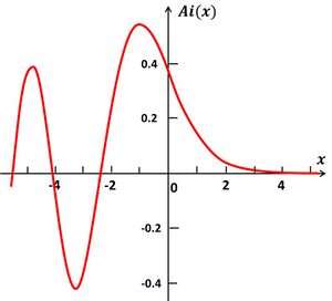
| + | where <math>Ai(\chi)</math> is the Airy function (Fig. C1), <math>\; Ai(\chi) = \Large\frac{1}{\pi}\normalsize \int_0^{\infty} \cos \big( \Large\frac{t^3}{3}\normalsize + \chi t \big) \, dt \; </math> and <math>\; \chi = \Big| \Large\frac{2}{S}\normalsize \Big|^{1/3} \big( \Large\frac{1}{2S}\normalsize + \zeta \Large\frac{S}{|S|}\normalsize \big) . </math> | ||
| + | |||
| + | For <math>S \rightarrow 0</math> the formula (C4) reduces to the Gaussian distribution <math>p(\zeta) = \Large\frac{1}{\sqrt{2 \pi}}\normalsize \exp(-\zeta^2 / 2) .</math> | ||
| − | + | {| border="0" align="center" | |
| − | + | |- | |
| − | + | | valign="top"| | |
| − | + | [[File:AiryFunction.jpg|thumb|left|300px|Fig. C1. The Airy function.]] | |
| + | | valign="top"| | ||
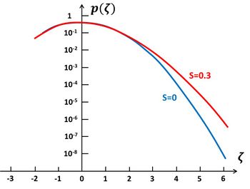
| + | [[File:DistributionNonLinearWaves.jpg|thumb|right|350px|Fig. C2. The probability density distributions Eq. (C3) for <math>S=0</math> (blue) and <math>S=0.3</math> (red).]] | ||
| + | |} | ||
| − | + | The Airy function <math>Ai(x)</math> oscillates for negative values of <math>x</math> (Fig. C1). The probability density (C4) can therefore take negative values for large negative values of <math>\zeta</math>, which is physically unrealistic. A positive skewness <math>S</math> corresponds to the usual situation of a peaked wave crest and shallow wave trough<ref name=LH/>. Large negative <math>\zeta</math> values (very deep wave troughs) are therefore highly improbable. The opposite holds for the unusual situation of negative skewness. Fig. C2 displays the probability density distributions for <math>S=0</math> (the linear case) and <math>S=0.3</math>. The probability of high wave peaks is much higher in the nonlinear case than in the linear case. | |
| − | + | Comments of David Fuhrman and Mathias Klahn on an earlier draft of this appendix are acknowledged. | |
| − | |||
| − | |||
| − | |||
| − | |||
| − | |||
| − | |||
| − | + | ==References== | |
| + | <references/> | ||
| − | |||
| − | |||
| − | |||
| − | |||
| + | {{2Authors | ||
| + | |AuthorID1=13331 | ||
| + | |AuthorFullName1=Mangor, Karsten | ||
| + | |AuthorName1=Karsten | ||
| + | |AuthorID2=120 | ||
| + | |AuthorFullName2=Job Dronkers | ||
| + | |AuthorName2=Dronkers J | ||
| + | }} | ||
| − | + | [[Category:Physical coastal and marine processes]] | |
| − | + | [[Category:Hydrodynamics]] | |
| − | [[ | ||
| − | |||
| − | |||
| − | |||
| − | [[ | ||
| − | |||
| − | |||
| − | |||
| − | |||
| − | |||
Latest revision as of 12:12, 23 November 2023
Because of the random nature of natural waves, a statistical description is normally always used. A fair approximation of the observed distribution of wave heights is given by the Rayleigh distribution. Statistical wave parameters are often calculated based on this distribution. The most commonly used variables in coastal engineering are described below.
Contents
Most commonly used variables in coastal engineering
Significant wave height
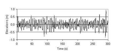
An example of a wave record representative for a certain sea state is shown in Fig. 1. The significant wave height, [math]H_s[/math], is the mean of the highest third of the waves; instead of [math]H_s[/math] the notation [math]H_{1/3}[/math] is also often used. [math]H_s[/math] represents well the average height of the highest waves in a wave group. The significant wave height can also be computed from the wave energy. For non-breaking waves it appears that [math]H_s \approx H_{m0} = 4 [\lt E\gt / (g \rho)]^{1/2}, [/math] where [math]H_{m0}[/math] is the spectral significant wave height. An explanation, definitions and formulas are given in appendix A.
Mean wave period
The mean wave period, [math]T_m[/math], is the mean of all wave periods in a time-series representing a certain sea state.
Peak wave period
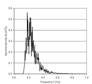
The peak wave period, [math]T_p[/math], is the wave period with the highest energy. The analysis of the distribution of the wave energy as a function of wave frequency [math]f=1/T[/math] for a time-series of individual waves is referred to as a spectral analysis. Wind wave periods (frequencies) often follow the so-called JONSWAP or Pierson-Moskowitz spectra (see appendix B). The peak wave period is extracted from the spectra. As a rule of thumb the following relation can be used, see Fig. 5[1]:
[math]T_p \approx 5 \sqrt{H_{m0}}. \qquad (1) [/math]
Mean wave direction
The mean wave direction, [math]\theta_m[/math], is defined as the mean of all the individual wave directions in a time-series representing a certain sea state.
Description of wave conditions
These various wave parameters are often calculated from continuous or periodic time-series of the surface elevations; typically the parameters are calculated once every one or three hours, whereby a new discrete time-series of the statistical wave parameters is constructed. This time-series is thereafter analyzed statistically to arrive at a condensed description of the wave conditions as follows:
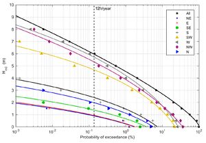
- Wave height distribution represented by [math]H_s[/math] vs. percentage of exceedance. This often follows a Weibull-distribution (see appendix A and the example in Fig. 3);
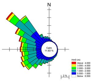
- Directional distribution of the wave heights, which is often presented in the form of a wave rose (see appendix B and the example in Fig. 4);
- Scatter diagram of [math]T_p[/math] vs. [math]H_s[/math] (example in Fig. 5).
Analyses of extreme wave conditions are performed on the basis of max. wave heights in single storm events or on the basis of annual max. wave heights. These analyses are often presented as exceedance probability vs. wave heights, see Fig. 6 for an example.
Further reading
- Mangor, K., Drønen, N.K., Kaergaard, K.H. and Kristensen, S.E. 2017. Shoreline Management Guidelines. DHI Water and Environment, 451pp. [2]
- Coastal Engineering Manual, part II, chapter 1. US Army Corps of Engineers (USACE), 2008
Appendix A: Rayleigh distribution
We consider a wave field [math]\eta(x,y,t)[/math] consisting of a superposition of [math]n[/math] independent, uncorrelated sinusoidal (i.e. linear) waves, with amplitudes [math]a_j[/math], radial frequencies [math]\omega_j[/math] and random phases [math]\phi_j[/math], originating from different nearby and remote regions. This superposition can be represented by
[math]\eta=Re[\sum_{j=1}^{n} a_j \exp(i\omega_j t + i\phi_j)]. \qquad (A1)[/math]
The statistical distribution of wave heights was derived by Longuet-Higgins (1952)[3] under a few specific conditions: (a) the radial frequencies [math]\omega_j[/math] of the random waves are grouped in a single narrow band around a central frequency [math]\omega[/math] such that [math]|\omega_j -\omega_j'|/ \omega \lt \lt 1[/math] for each [math]j, j' \, ; \;[/math] (b) the slowly varying numbers [math]\; a=\sum_{j=1}^{n} a_j \cos \big( \phi_j + (\omega_j - \omega)t \big), \, b=\sum_{j=1}^{n} a_j \sin\big( \phi_j + (\omega_j - \omega)t \big) \;[/math] are statistically independent and normally (Gaussian) distributed. Under these conditions the expression (A1) can be approximated for the time interval [[math]-\pi / \omega \lt t\lt \pi / \omega[/math]] by
[math]\eta \approx \frac{1}{2} H \, \cos(\omega t+ \phi) , \quad H = 2 \sqrt{a^2 + b^2} , \quad \phi = \tan^{-1} (b/a) . \qquad (A2)[/math]
A well-known mathematical theorem[4] states that the length of a vector with Gaussian distributed components follows the Rayleigh distribution. In this case the vector length is the wave height [math]H[/math] and the components are the random numbers [math]\sqrt{2}a, \sqrt{2}b[/math]. The Rayleigh probability density function [math]p_R(H)[/math] for the wave height [math]H[/math] reads:
[math]p_R(H) = \Large\frac{2H}{H_{rms}^2}\normalsize \exp\Large (–(\frac{H}{H_{rms}})^2)\normalsize . \qquad (A3)[/math]
The root mean square wave height (also called mean energy wave height) [math]H_{rms}[/math] is related to the average wave energy [math]\lt E\gt [/math]:
[math] H_{rms}^2 = \int_0^{\infty} p_R(H) H^2 dH =\Large\frac{8}{g \rho}\normalsize \lt E\gt . \qquad (A4)[/math]
The average wave energy is defined as [math]\lt E\gt = g \rho \, m_0 \equiv g \rho \lt (\, \eta(t)-\lt \eta\gt )^2\gt [/math], where [math]g[/math] is the gravitational acceleration, [math]\rho[/math] the seawater density and where [math]\; \lt …\gt \; [/math] designates the average over a period much longer than the characteristic wave periods. Not considering wave set-up / set-down implies [math]\lt \eta\gt =0[/math].
The average wave height [math]\lt H\gt [/math] is related to the root mean square wave height [math]H_{rms}[/math] by
[math]\lt H\gt = \int_0^{\infty} p_R(H) H dH = \Large\frac{\sqrt{\pi}}{2}\normalsize H_{rms} \approx 0.89 H_{rms} .\qquad (A5)[/math]
The cumulative Rayleigh distribution (probability of wave height [math]\lt H[/math]) is given by
[math]P_R(H)=\int_0^H p_R(H')dH' = 1-\exp\Large (-(\frac{H}{H_{rms}})^2)\normalsize .\qquad (A6) [/math]
Assuming that wave heights are Reynolds distributed, relations can be derived between different wave parameters that are often used in practice. For the derivation of the significant wave height [math]H_s \equiv H_{1/3}[/math] (the mean of the highest 1/3-part of the waves) we first determine the lowest height of the highest 1/3-part of the waves, [math]H_3[/math], from the condition [math]P_R(H_3)=2/3[/math], yielding [math]H_3=H_{rms} \sqrt{\ln(3)}[/math]. The significant wave height is then related to the root mean square wave height by
[math]H_s=\Large\frac{\int_{H_3}^{\infty} p_R(H)HdH}{\int_{H_3}^{\infty} p_R(H)dH }\normalsize = 3 \, \int_{H_3}^{\infty} p_R(H)HdH \approx 1.6 \lt H\gt = 1.42 H_{rms}. \qquad (A7)[/math]
From Eqs. (A4) and (A7), it follows that the significant wave height [math]H_s[/math] is related to the average wave energy [math]\lt E\gt [/math] by
[math]H_s \approx H_{m0} \equiv 4 \Large \sqrt{ \frac{\lt E\gt }{g \rho}}\normalsize \equiv 4 \sqrt{m_0}. \qquad(A8)[/math]
Extreme wave heights can be derived from the Rayleigh distribution in a similar way. For example, the mean of the 1% highest waves is given by
[math]H_{1/100} \approx 1.52 H_s . \qquad (A9)[/math]
The Rayleigh distribution has been derived under the rather restrictive conditions ((a) and (b)). Since the Rayleigh distribution does not put a limit on the wave height, it allows for unrealistic high waves. When compared with wave height statistics obtained from field observations, it appears that the Rayleigh distribution tends to overestimate wave heights. This overestimation is greatest (more than 8%) for high long-period waves. Overestimation of the wave height is mainly due to wave breaking, which is related to increasing sharpness of wave peaks in deep water or to depth-induced wave breaking in shallow water[5]. A broad-banded instead of a narrow-banded wave spectrum can be another reason for wave height overestimation by the Rayleigh distribution[6]. Unlike wave height, wave crest height is generally underestimated by the Rayleigh distribution. The main reason for underestimating the wave crest height is the neglect of nonlinearity in the wave field[7]. Nonlinearity generates so-called 'skewed' waves: the wave shape changes from sinusoidal to more peaked with narrow wave crests and more shallow and wide wave troughs[8]. The conditions underlying the Rayleigh distribution are not satisfied in the case of significant nonlinearity, because the wave components in Eq. A1 are not random but correlated to generate a systematic deviation from the sinusoidal shape[9][10], see Appendix C: Distribution of nonlinear waves.
The Weibull distribution is one of the proposed alternatives to the Rayleigh distribution. The Weibull distribution reads [11] :
[math]p_W(H)=\Large\frac{m}{\lambda}(\frac{H}{\lambda})^{(m-1)}\normalsize \exp\Large (–(\frac{H}{\lambda})^{m}) \normalsize . \qquad (A10)[/math]
The Rayleigh distribution corresponds to the Weibull distribution for [math]m=2, \; \lambda=H_{rms}[/math]. The Weibull distribution has an additional parameter ([math]m[/math]) that allows suppression of the highest waves for [math]m\gt 2[/math] and an optimum adjustment to the observed wave data.
This is especially relevant for shallow-water waves, which are truncated due to depth-induced wave breaking (see Breaker index). Because of this truncation, the random numbers [math]a[/math] and [math]b[/math] in Eq. (2) are not Gaussian distributed; the wave height therefore does not follow a Rayleigh distribution. For this situation, alternative distributions have been proposed, for example by Battjes and Groenendijk (2000)[12]. According to this study, a Weibull distribution with [math]m=3.6[/math] should be used above a certain threshold, [math]H_{tr}[/math] (threshold for depth-induced wave breaking). This implies that the relationships (A7-A9) are not valid in shallow water. For example, if [math]H_{tr}\lt H_s[/math] (i.e. very shallow water), Eq. (A9) should be replaced by [12]
[math]H_{1/100} \approx 1.28 H_s . \qquad (A11)[/math]
Flume experiments of shallow-water wave transformation show that the value of [math]m[/math] is not constant but varies over the surf zone slope (gradual increase followed by decrease[13]).
Appendix B: Frequency spectrum
A wave record can further be characterized by its frequency spectrum. The energy density spectrum of a sea state is generally designated by [math]E(f)[/math]. The total energy is given by
[math]\lt E\gt =\int_0^{\infty} E(f)df . \qquad (B1)[/math]
The wave frequency spectrum can be determined from a wave record [math]\eta(t)[/math] by using a Fourier transform as follows: The wave energy averaged over a period [math][-T/2 \lt (t -t_0)\lt T/2] [/math] is given by [math]\lt E\gt =\frac{g \rho}{T} \int_{-T/2}^{T/2} (\eta(t-t_0) - \lt \eta\gt )^2 dt[/math], where [math]\lt \eta\gt [/math] is the mean value. Inserting in this expression the Fourier development of [math](\eta(t-t_0) - \lt \eta\gt )[/math] gives
[math]\lt E\gt =\sum_{k=1}^{\infty} E(f_k) \Delta f , \quad f_k=k \Delta f, \; \Delta f = \frac{1}{T} , \quad E(f_k) \Delta f =\frac{g \rho}{8} |H_k|^2 , \quad H_k = \frac{4}{T} \int_{-T/2}^{T/2} (\eta(t-t_0)-\lt \eta\gt ) e^{-2 i \pi f_k t} dt . [/math]
The wave frequency spectrum can also be determined by modelling the wind-induced wave field in a large source area. Empirical formulas have been established for fully developed wave fields under constant wind stress. For deep water without fetch restriction, it is recommended to use the adapted Pierson-Moskowitz frequency distribution [math]E_{PM}[/math] [14]:
[math]E_{PM}(f) = \alpha_{PM} \Large\frac{\lt E\gt }{f_p}(\frac{f_p}{f})^4 e^{-(\frac{f_p}{f})^4}\normalsize . \qquad (B2)[/math]
For the average wave energy [math]\lt E\gt [/math] and the peak frequency [math]f_p[/math] the following empirical expressions are found:
[math]\lt E\gt \approx 0.005 \rho g^{-1} U_{10}^4\; , \; f_p \approx 0.123 g U_{10}^{-1} \; ,[/math]
where [math]g[/math] is the gravitational acceleration and [math]U_{10}[/math] the wind velocity at 10 m above the sea surface. For the coefficient [math]\alpha_{PM}[/math] a usual value is [math]\alpha_{PM} \approx 3.26[/math].
For fetch-limited seas, the spectrum is more strongly peaked around the peak frequency. For this situation, the adapted empirical JONSWAP spectrum can be used. It has the form
[math]E_{JWP} = \alpha_{JWP} \Large\frac{\lt E\gt }{f_p}(\frac{f_p}{f})^4 e^{-(\frac{f_p}{f})^4}\normalsize \gamma^\delta \;, \quad \delta =e^{-\Large\frac{1}{2}\Large(\frac{(f/f_p)-1}{\sigma})^2}\normalsize , \qquad (B3)[/math],
where the parameters [math]\alpha_{JWP}, \gamma, \sigma, f_p[/math] depend on the wind velocity and the fetch length and should be fitted to the wave data. The peak enhancement factor [math]\gamma[/math] can take values between 1 and 7 depending on the ocean region and depending on calm of stormy weather conditions. For [math]\gamma=1[/math] the Pierson-Moskowitz and JONSWAP spectra are the same. The most usual value is [math]\gamma=3.3[/math], but a lower value (between 1 and 2) is probably more appropriate for most ocean regions[15].
Different characteristic wave periods can be derived from the wave spectrum: the significant wave period [math]T_{01}[/math], the mean wave period [math]T_{02}[/math] and the mean energy period [math]T_E \equiv T_{m-1,0}[/math]. They are given by the expressions
[math]T_{01} = \Large\frac{\int_0^{\infty} E(f)df}{\int_0^{\infty} E(f)fdf }\normalsize, \quad T_{02} = \Large \sqrt{\frac{\int_0^{\infty} E(f)df}{\int_0^{\infty} E(f) f^2 df }}\normalsize, \quad T_E \equiv T_{m-1,0} = \Large\frac{\int_0^{\infty} E(f) f^{-1} df}{\int_0^{\infty} E(f)df }\normalsize \; .\qquad (B4) [/math]
The peak frequency [math]f_p=T_p^{-1}[/math] is related to the mean energy period [math]T_E[/math]. Fitting the Pierson-Moskowitz distribution (B2) to field data yields [math]T_E/T_p \approx 0.85 [/math]; fitting the JONSWAP distribution (B3) yields [math]T_E/T_p \approx 0.9 [/math]. The ratio [math]T_E/T_p[/math] can also be derived directly from field data.
The periods defined by Eq. (B4) can be misleading when the frequency spectrum has multiple peaks corresponding to different kinds of waves, for example short-period sea waves, long-period swell waves and infragravity waves with the period of wave groups. In this case, the separate periods can be determined by integrating the spectrum over frequency bandwidths associated with the different kinds of waves. An analysis of hindcasted wave data for the US Atlantic and Pacific coasts [16] yielded an overall value of [math]T_E/T_p = 0.81 - 0.85 [/math]. Considering separately wind wave-dominated data and swell-dominated data, the resulting values were [math]T_E/T_p = 0.85 -0.88[/math] for wind waves and [math]T_E/T_p = 0.93 – 0.97[/math] for swell waves.
In an irregular wave field, waves may come from different directions. The wave incidence direction is an important parameter for sediment transport in the coastal zone. Waves originating from different areas may have different spectra. The directional spread of incoming waves for a particular wave frequency can be represented by a distribution function [math]D(f,\theta)[/math], where [math]\theta[/math] is the wave incidence angle. We then have
[math]\lt E\gt \equiv \int_0^{\infty} \int_0^{2 \pi} S(f, \theta) df d \theta \equiv \int_0^{\infty} \int_0^{2 \pi} E(f) \, D(f, \theta) df d \theta \; ,\quad \int_0^{2 \pi} D(f, \theta) d \theta =1 \; .\qquad (B5) [/math]
The directional wave spectrum [math]S(f, \theta)[/math] can be derived from directional wave buoys. In practice, it is often obtained by numerical modelling of the wave field in the major source area.
Appendix C: Distribution of nonlinear waves
Here we reproduce an expression for the probability density distribution [math]p(\zeta)[/math] of the normalized surface elevation [math]\zeta[/math] of nonlinear waves following the derivation by Fuhrman, Klahn and Zhai (2023[17]).
In appendix A we considered a wave field consisting of sinusoidal waves. However, waves incident on the coast are typically skewed as a result of nonlinear interactions and hence cannot be considered statistically independent. So here we consider a wave field
[math]\zeta = \zeta_1 + \zeta_2 + \zeta_3 + ….. , \qquad (C1)[/math]
where the first order field [math]\zeta_1[/math] consists of densely distributed but uncorrelated waves as in (A1). These sinusoidal first order waves are modified by nonlinear interactions which generate higher harmonic waves [math]\zeta_2[/math] of second order ([math]O(\epsilon), \, \epsilon \lt \lt 1[/math]) and harmonic waves, [math]\zeta_3, \zeta_4, …[/math] of higher order ([math]O(\epsilon^k), k \ge 2[/math]). The small parameter [math]\epsilon[/math] is a measure of the average wave steepness. The mean surface elevation [math]\lt \zeta\gt [/math] is taken equal to zero and the wave field [math]\zeta[/math] is normalized such that [math]\lt \zeta^2 \gt = 1[/math].
No theoretical analytical expression of [math]p(\zeta)[/math] exists for nonlinear waves in general, but Fuhrman et al. 2023[17] have shown that an exact expression can be obtained when terms of order [math]\epsilon^k, \; k \ge 2[/math] are ignored. This implies that the wave skewness [math]S \equiv \lt \zeta^3\gt [/math] is given by [math]S = \lt \zeta_1^2 \zeta_2\gt [/math]. Also to order [math]\epsilon[/math], expressions can be derived for the higher moments of [math]\zeta[/math]:[8]
[math] \lt \zeta^{2n}\gt = \Large\frac{2n!}{2^n n!}\normalsize \; , \quad \lt \zeta^{2n+1}\gt = \Large\frac{S}{6}\frac{(2n+1)!}{2^{n-1} (n-1)!}\normalsize . \qquad (C2)[/math]
Now consider the function [math]M_{\zeta}(s) \equiv \lt \exp(i \zeta s) \gt \equiv \int_{-\infty}^{\infty} p(\zeta) \exp(i \zeta s) ds [/math]. The probability density function [math]p(\zeta)[/math] can be found from the inverse Fourier transform
[math]p(\zeta) = \Large\frac{1}{2 \pi}\normalsize \int_{-\infty}^{\infty} \exp \big( \ln(M_{\zeta}(is)) - i \zeta s \big) ds . \qquad (C3)[/math]
In order to evaluate this expression [math]M_{\zeta}(s)[/math] is developed into a Taylor series, [math]M_{\zeta}(s) = \sum_{n=0}^{\infty} \Large\frac{s^n}{n!}\normalsize \lt \zeta^n\gt ,[/math] this series is substituted in the Taylor expansion [math]\ln(M_{\zeta}(s)) = - \sum_{n=1}^{\infty} \Large\frac{(-1)^n}{n}\normalsize (M_{\zeta}(s) -1)^n [/math]. Ignoring all terms of order [math]\epsilon^2[/math] and higher and using the expressions (C2) gives the result [math]\; \ln(M_{\zeta}(s)) = \Large\frac{1}{2}\normalsize s^2 + \Large\frac{1}{6}\normalsize S s^3 . [/math] It is emphasized that the exact skewness [math]S \equiv \lt \zeta^3\gt [/math] is utilized here.
Substitution in Eq. (C3) yields an expression for the distribution [math]p(\zeta)[/math]. Evaluating this integral gives
[math]p(\zeta) = \Big| \Large\frac{2}{S}\normalsize \Big|^{1/3} \exp \big( \Large\frac{1}{3 S^2}+\frac{\zeta}{S}\normalsize \big) Ai(\chi) , \qquad (C4)[/math]
where [math]Ai(\chi)[/math] is the Airy function (Fig. C1), [math]\; Ai(\chi) = \Large\frac{1}{\pi}\normalsize \int_0^{\infty} \cos \big( \Large\frac{t^3}{3}\normalsize + \chi t \big) \, dt \; [/math] and [math]\; \chi = \Big| \Large\frac{2}{S}\normalsize \Big|^{1/3} \big( \Large\frac{1}{2S}\normalsize + \zeta \Large\frac{S}{|S|}\normalsize \big) . [/math]
For [math]S \rightarrow 0[/math] the formula (C4) reduces to the Gaussian distribution [math]p(\zeta) = \Large\frac{1}{\sqrt{2 \pi}}\normalsize \exp(-\zeta^2 / 2) .[/math]
The Airy function [math]Ai(x)[/math] oscillates for negative values of [math]x[/math] (Fig. C1). The probability density (C4) can therefore take negative values for large negative values of [math]\zeta[/math], which is physically unrealistic. A positive skewness [math]S[/math] corresponds to the usual situation of a peaked wave crest and shallow wave trough[8]. Large negative [math]\zeta[/math] values (very deep wave troughs) are therefore highly improbable. The opposite holds for the unusual situation of negative skewness. Fig. C2 displays the probability density distributions for [math]S=0[/math] (the linear case) and [math]S=0.3[/math]. The probability of high wave peaks is much higher in the nonlinear case than in the linear case.
Comments of David Fuhrman and Mathias Klahn on an earlier draft of this appendix are acknowledged.
References
- ↑ Mangor, K., Drønen, N.K., Kaergaard, K.H. and Kristensen, S.E. 2017. Shoreline Management Guidelines. DHI Water and Environment, 451pp.
- ↑ https://www.dhigroup.com/upload/campaigns/ShorelineManagementGuidelines_Feb2017.pdf
- ↑ Longuet-Higgins, M.S. 1952. On the statistical distribution of sea waves. Journal of Marine Research 11: 245-266
- ↑ https://en.wikipedia.org/wiki/Rayleigh_distribution
- ↑ Karmpadakis, I. and Swan, C. 2022. A new crest height distribution for nonlinear and breaking waves in varying water depths. Ocean Engineering 266, 112972
- ↑ Karmpadakis, I., Swan, C. and Christou, M. 2022. A new wave height distribution for intermediate and shallow water depths. Coastal Engineering 175, 104130
- ↑ Tayfun, M.A. 1980. Narrow-Band Nonlinear Sea Waves. J. Geophysical Research 85(C3): 1548-1552
- ↑ 8.0 8.1 8.2 Longuet-Higgins, M.S. 1963. The effect of non-linearities on statistical distributions in the theory of sea waves. J. Fluid Mech. 17: 459-480
- ↑ Casas‐Prat, M. and Holthuijsen, L. H. 2010. Short‐term statistics of waves observed in deep water. J. Geophys. Res. 115, C09024
- ↑ Karmpadakis, I., Swan, C. and Christou, M., 2020. Assessment of wave height distributions using an extensive field database. Coastal Engineering 157, 103630
- ↑ https://en.wikipedia.org/wiki/Weibull_distribution
- ↑ 12.0 12.1 Battjes, J.A. and Groenendijk, H.W. 2000. Wave height distributions on shallow foreshores. Coastal Engineering 40: 161-182
- ↑ Xu, J., Liu, S., Li, J. and Jia, W. 2021. Experimental study of wave height, crest, and trough distributions of directional irregular waves on a slope. Ocean Engineering 242: 110136
- ↑ The Rock Manual. The use of rock in hydraulic engineering (2nd edition).CIRIA. London, 2007
- ↑ Mazzaretto, O.M., Menendez, M. and Lobeto, H. 2022. A global evaluation of the JONSWAP spectra suitability on coastal areas. Ocean Engineering 266, 112756
- ↑ Ahn, S. 2021. Modeling mean relation between peak period and energy period of ocean surface wave systems. Ocean Engineering 228, 108937
- ↑ 17.0 17.1 Fuhrman, D.R., Klahn, M. and Zhai, Y. 2023. A new probability density function for the surface elevation in irregular seas. J. Fluid Mech. 970, A38
Please note that others may also have edited the contents of this article.
|
