File list
This special page shows all uploaded files.
| Date | Name | Thumbnail | Size | Description | Versions |
|---|---|---|---|---|---|
| 09:57, 15 September 2016 | GiovanniFig3.jpg (file) |  |
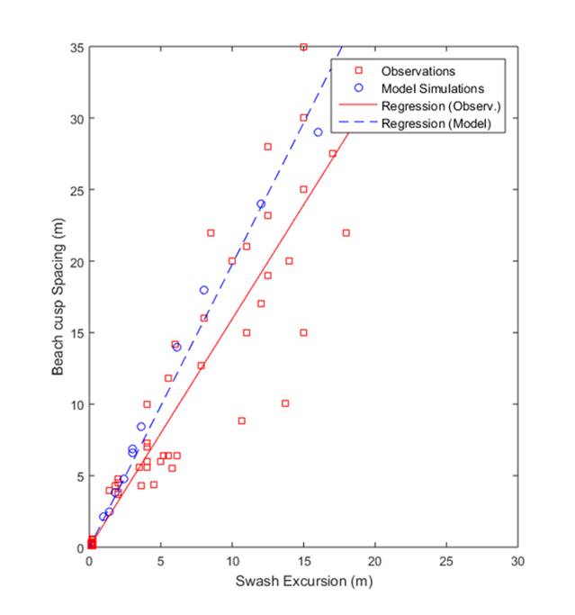
27 KB | Figure 3. Beach cusp spacing as a function of swash excursion for measurements and numerical simulations. | 1 |
| 09:56, 15 September 2016 | GiovanniFig2.jpg (file) |  |
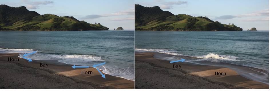
40 KB | Figure 2. Flow circulation over beach cusps. | 1 |
| 09:37, 15 September 2016 | GiovanniFig4.jpg (file) |  |
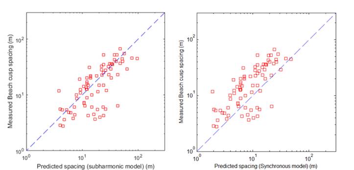
23 KB | Figure 4. Measured beach cusp spacing versus the spacing predicted assuming the presence of subharmonic (left panel) or synchronous (right panel) standing edge waves. | 1 |
| 15:35, 14 September 2016 | CocoFig4.jpg (file) |  |
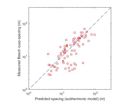
20 KB | Figure 4: Measured beach cusp spacing versus the spacing predicted assuming the presence of subharmonic standing edge waves. | 1 |
| 15:35, 14 September 2016 | CocoFig3.jpg (file) |  |
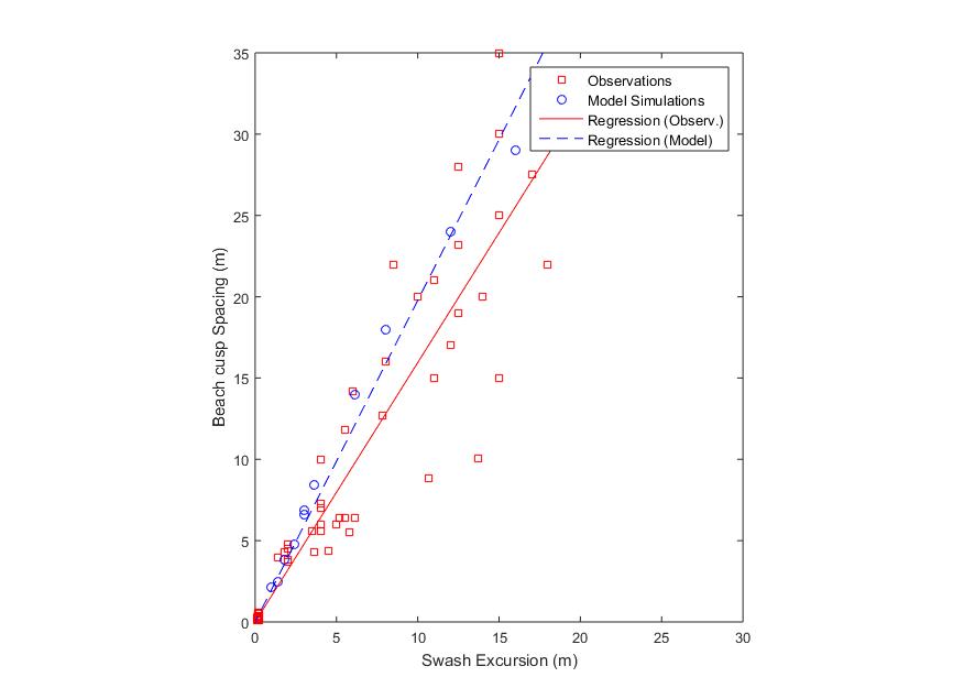
31 KB | Figure 3: Beach cusp spacing as a function of swash excursion for measurements (field and laboratory) and numerical simulations. | 1 |
| 15:34, 14 September 2016 | Fig2.jpg (file) |  |
40 KB | Figure 2: Snapshots of flow circulation over beach cusps. | 1 |
| 15:33, 14 September 2016 | CocoFig1.jpg (file) |  |
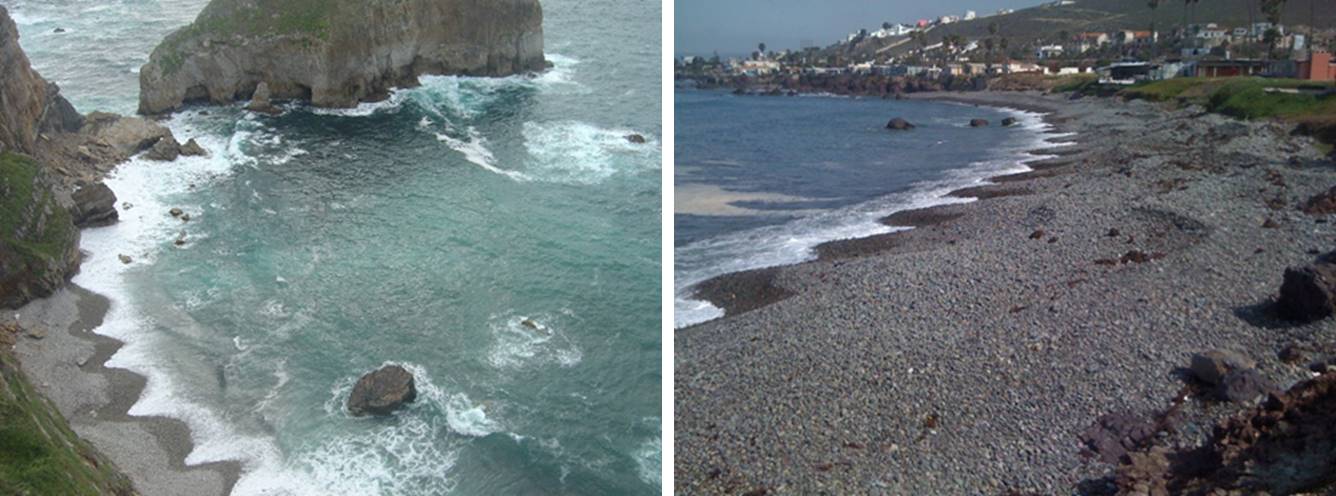
101 KB | Figure 1: Beach cusps | 1 |
| 15:27, 13 September 2016 | LucianaTable1.jpg (file) |  |
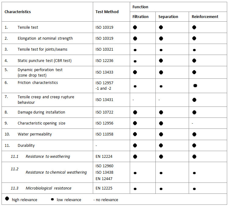
122 KB | Table 1: Characteristics of geotextiles and geotextile-related products according to functions and test methods. | 1 |
| 15:26, 13 September 2016 | LucianaFig1.jpg (file) |  |
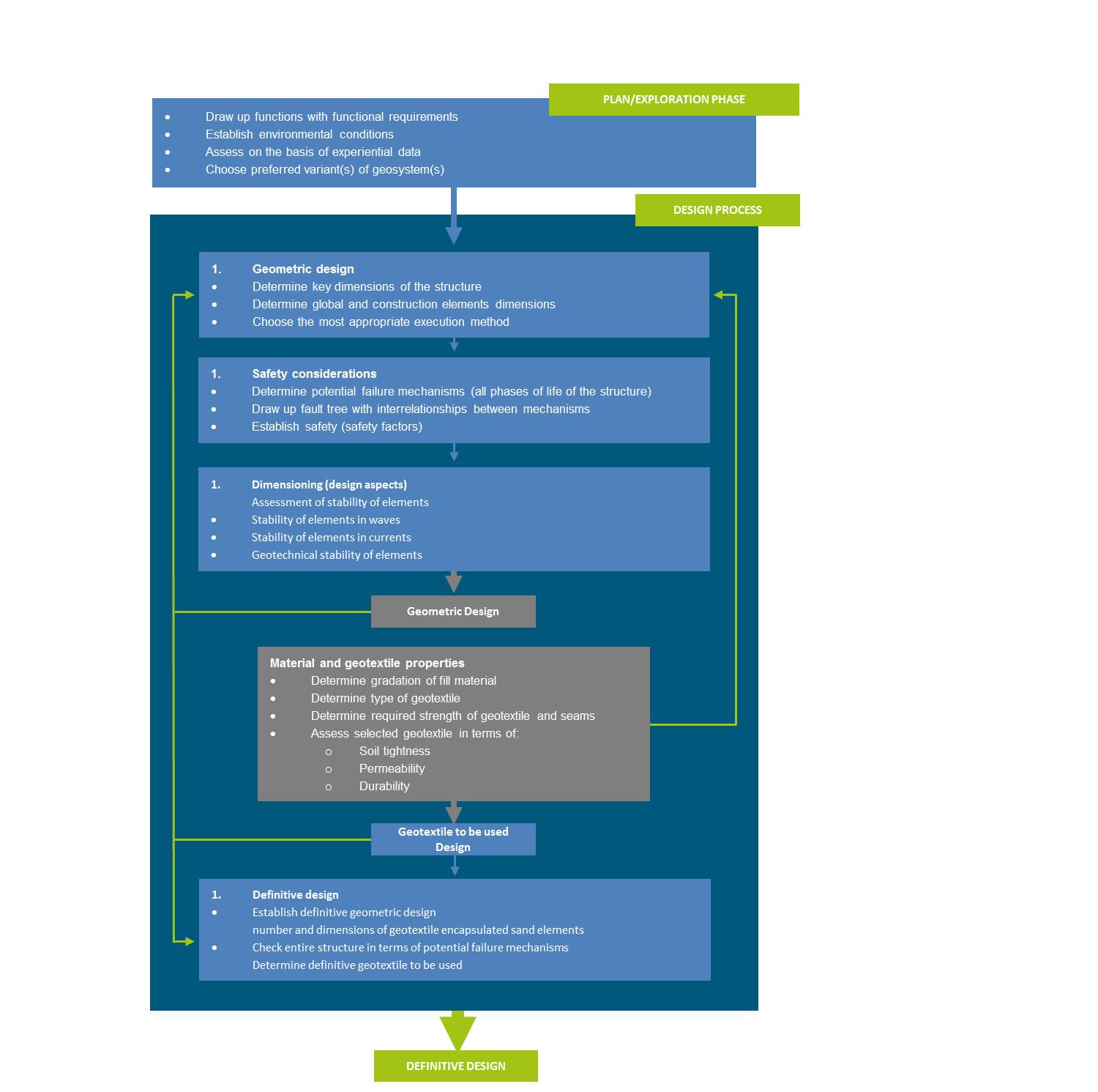
124 KB | Fig 1. Iterative design process for sand-filled geosystems | 1 |
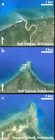
| 17:56, 18 August 2016 | NienhuisFig3.jpg (file) |  |
33 KB | Figure 3: Three deltas with varying wave influence. | 1 |
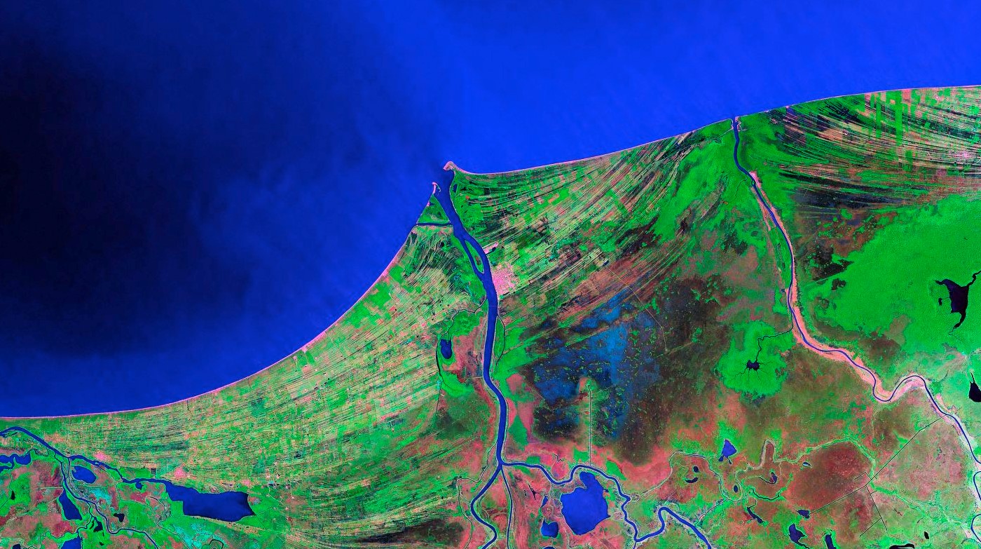
| 17:49, 18 August 2016 | NienhuisFig2.jpg (file) |  |
357 KB | Figure 2: The Rio Grijalva in Mexico. | 1 |
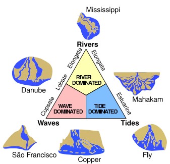
| 17:48, 18 August 2016 | NienhuisFig1.jpg (file) |  |
29 KB | Figure 1: The ternary diagram of delta morphology. | 1 |
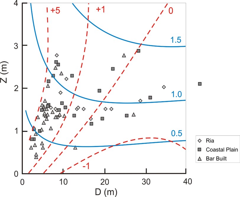
| 22:44, 5 August 2016 | PrandleFig14.jpg (file) |  |
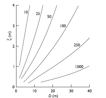
67 KB | Figure 14. Tidal current amplitude, U, as a function of depth, D and tidal elevation amplitude, Z, based on bed friction coefficient, f= 0.0025. | 1 |
| 22:43, 5 August 2016 | PrandleFig13.jpg (file) |  |
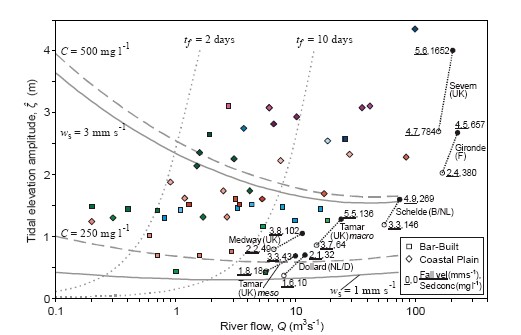
40 KB | Figure 13. ‘Equilibrium’ values of sediment concentrations and fall velocities. | 1 |
| 22:42, 5 August 2016 | PrandleFig12.jpg (file) |  |
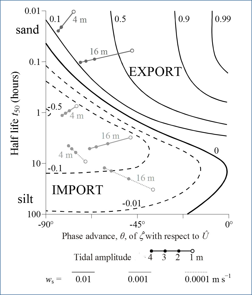
123 KB | Figure 12. Spring-neap variability in import vs export of sediments. | 1 |
| 22:41, 5 August 2016 | PrandleFig11.jpg (file) |  |
41 KB | Figure 11. Schematic of dynamical and sedimentary components integrated into the analytical emulator. | 1 |
| 22:40, 5 August 2016 | PrandleFig10.jpg (file) |  |
49 KB | Figure 10. Bathymetric Zone. | 1 |
| 22:38, 5 August 2016 | PrandleFig9.jpg (file) |  |
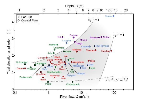
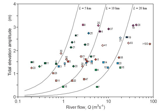
30 KB | Figure 9. Theoretical and observed estuarine lengths L as function of (Q, Z). | 1 |
| 22:38, 5 August 2016 | PrandleFig8.jpg (file) |  |
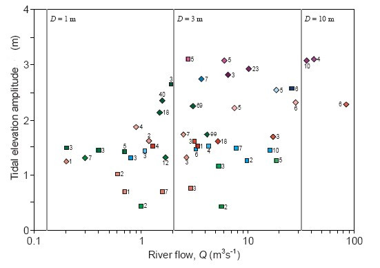
25 KB | Figure 8. Observed vs. theoretical estuarine depths at the mouth, D (m), as function of (Q, Z). | 1 |
| 22:37, 5 August 2016 | PrandleFig7.jpg (file) |  |
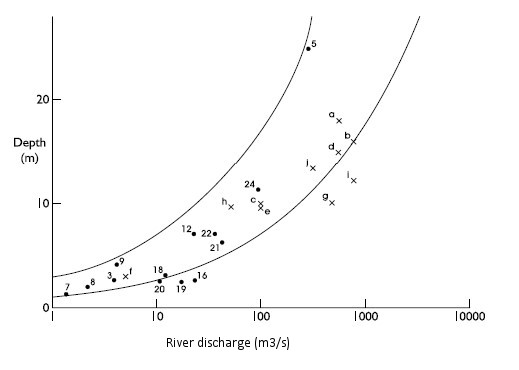
16 KB | Figure 7. Theoretical envelope : Depth at the mouth as a function of river flow. | 1 |
| 22:36, 5 August 2016 | PrandleFig6.jpg (file) |  |
17 KB | Estuarine length, L (km), as a function of (D, Z) , with f=0.0025. | 1 |
| 22:36, 5 August 2016 | PrandleFig5.jpg (file) |  |
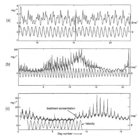
48 KB | Figure 5. Observed SPM (suspended matter concentration) and current time-series in: (a) Dover Straits, (b) Mersey Estuary and (c) Holderness Coast. | 1 |
| 22:35, 5 August 2016 | PrandleFig4.jpg (file) |  |
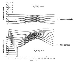
23 KB | Figure 4. Model simulations of SPM over a spring-neap tidal cycle. | 1 |
| 22:34, 5 August 2016 | PrandleFig3.jpg (file) |  |
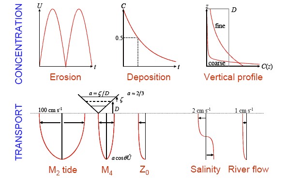
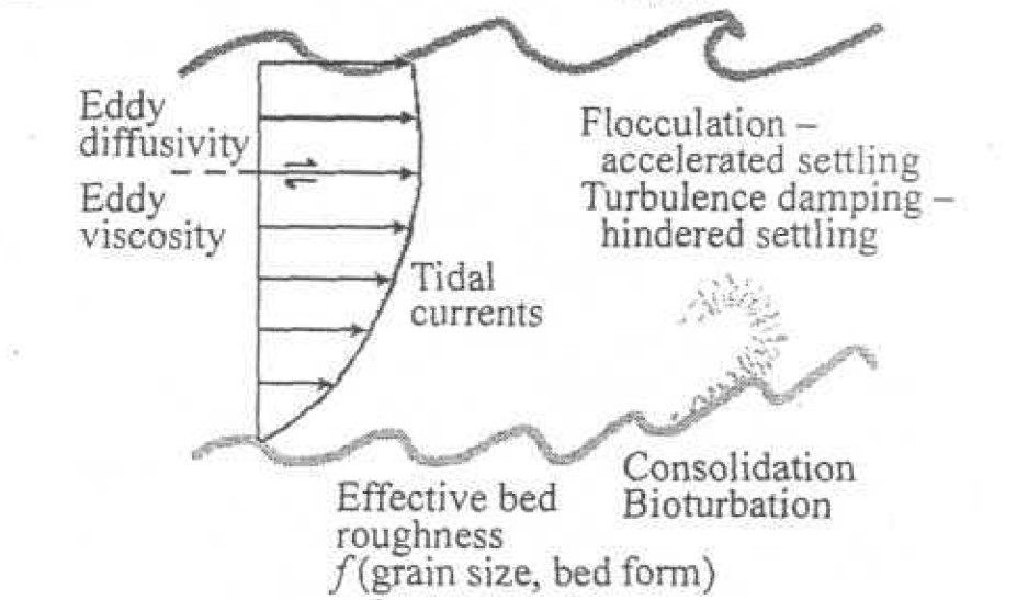
75 KB | Figure 3. Processes determining sediment erosion, transport and deposition. | 1 |
| 22:33, 5 August 2016 | PrandleFig2.jpg (file) |  |
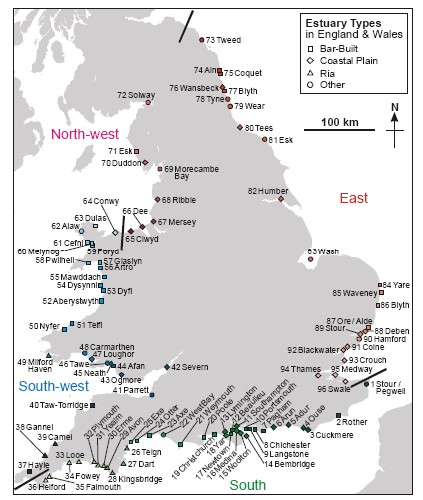
59 KB | Figure 2. Estuaries of England and Wales. | 1 |
| 22:32, 5 August 2016 | PrandleFig1.jpg (file) |  |
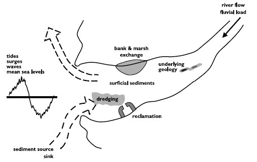
26 KB | Figure 1: Schematic of major factors influencing estuarine bathymetry. | 1 |
| 22:35, 4 August 2016 | CamFig3.jpg (file) |  |
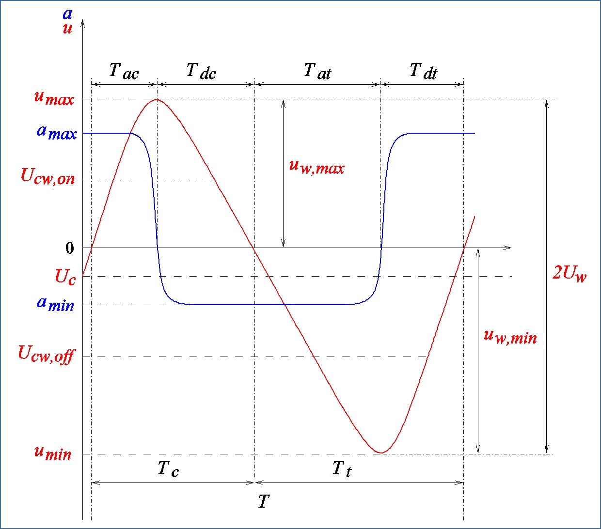
140 KB | Schematic view of the instantaneous velocity and acceleration variation for a bore over a wave period and in the direction of the waves. | 1 |
| 22:23, 4 August 2016 | CamFig2.jpg (file) |  |
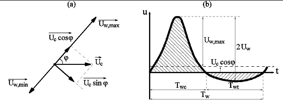
59 KB | Bottom velocity profile in the direction of the wave propagation | 1 |
| 22:22, 4 August 2016 | CamFig1.jpg (file) |  |
83 KB | Profile of the time-dependent velocity (a) and bed shear stress (b) in the wave direction | 1 |
| 07:57, 7 July 2016 | WesternScheldt.jpg (file) |  |
214 KB | Western Scheldt and Scheldt estuary | 2 |
| 16:25, 6 July 2016 | Columbia.jpg (file) |  |
241 KB | Columbia River estuary | 1 |
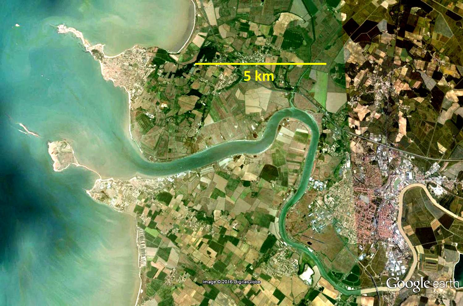
| 16:24, 6 July 2016 | Charente.jpg (file) |  |
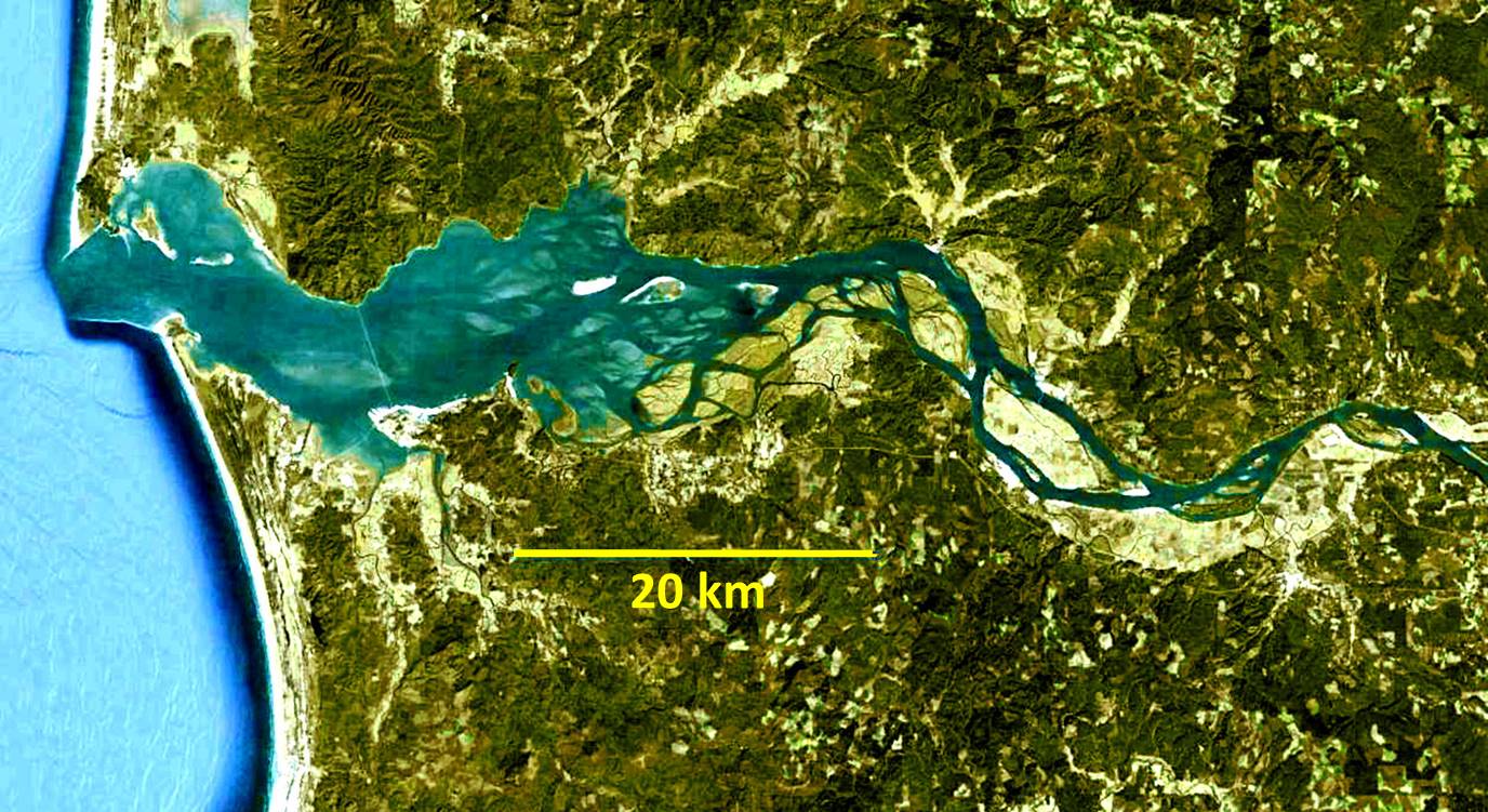
249 KB | Charente estuary | 1 |
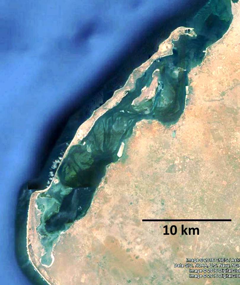
| 16:24, 6 July 2016 | Mussulo.jpg (file) |  |
86 KB | Mussulo Lagoon | 1 |
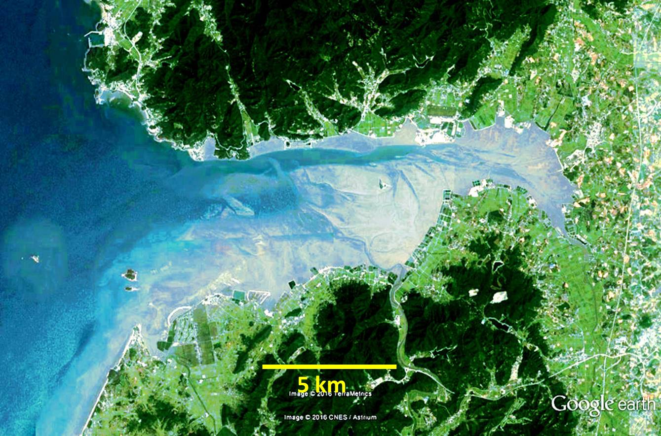
| 16:22, 6 July 2016 | Gomso.jpg (file) |  |
217 KB | Gomso Bay | 1 |
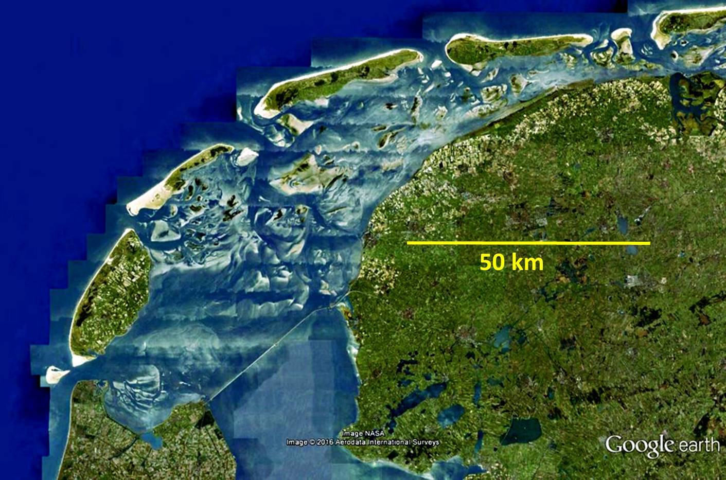
| 16:21, 6 July 2016 | Wadden.jpg (file) |  |
209 KB | Western Wadden Sea | 1 |
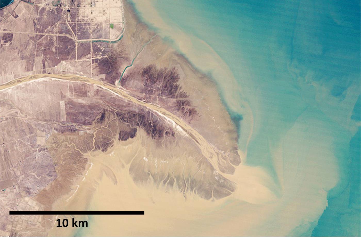
| 16:20, 6 July 2016 | Yellow.jpg (file) |  |
118 KB | Yellow River delta | 1 |
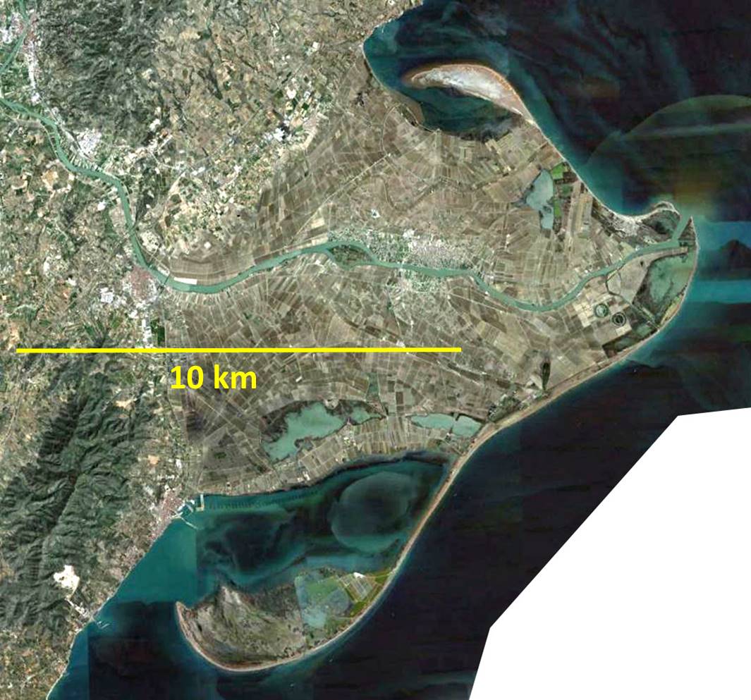
| 16:20, 6 July 2016 | Ebro.jpg (file) |  |
156 KB | Ebro delta | 1 |
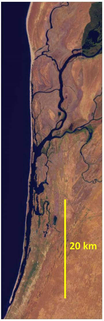
| 16:18, 6 July 2016 | Senegal.jpg (file) |  |
47 KB | Senegal River delta | 1 |
| 16:18, 6 July 2016 | Mahakam.jpg (file) |  |
135 KB | Mahakam River delta | 1 |
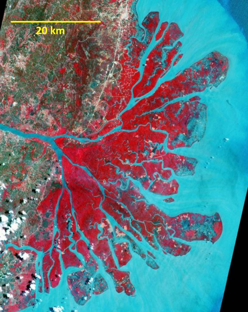
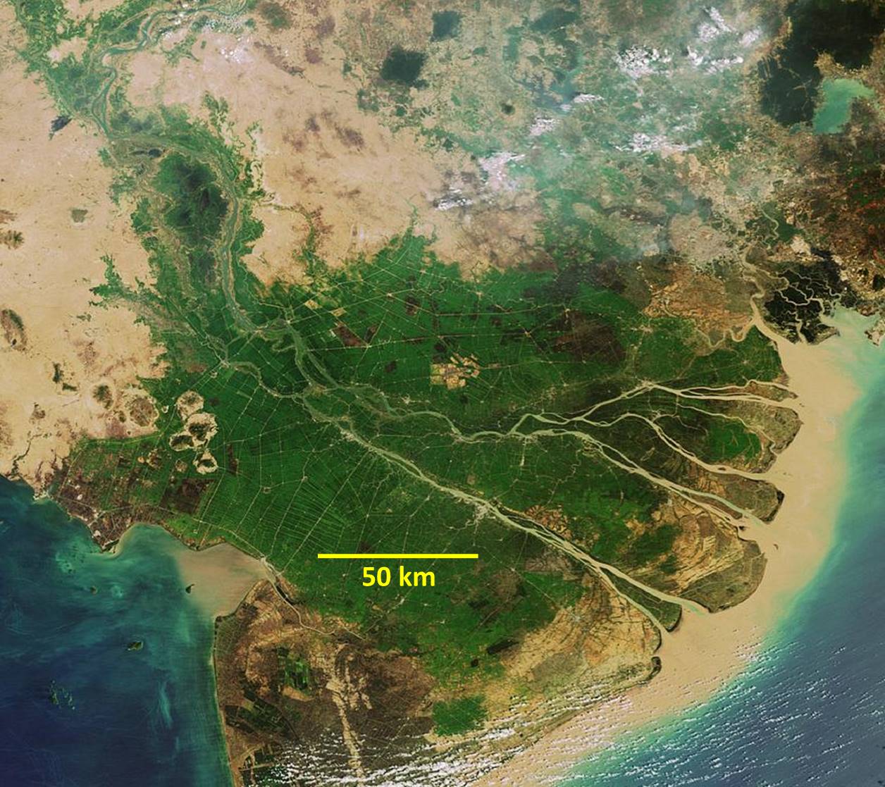
| 16:17, 6 July 2016 | Mekong.jpg (file) |  |
233 KB | Mekong delta | 1 |
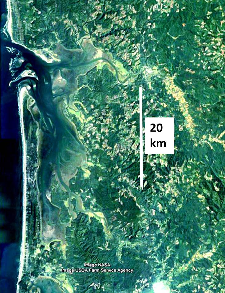
| 16:16, 6 July 2016 | Willapa.jpg (file) |  |
151 KB | Willapa Bay | 1 |
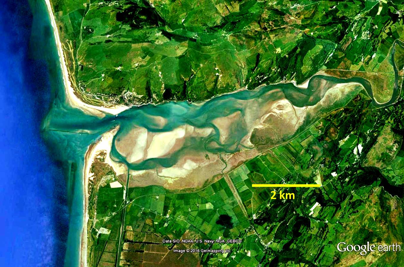
| 16:16, 6 July 2016 | Dyfi.jpg (file) |  |
238 KB | Dyfi estuary | 1 |
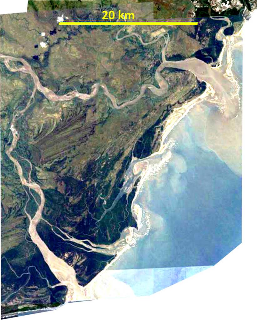
| 16:15, 6 July 2016 | Zambezi.jpg (file) |  |
120 KB | Zambezi River delta | 1 |
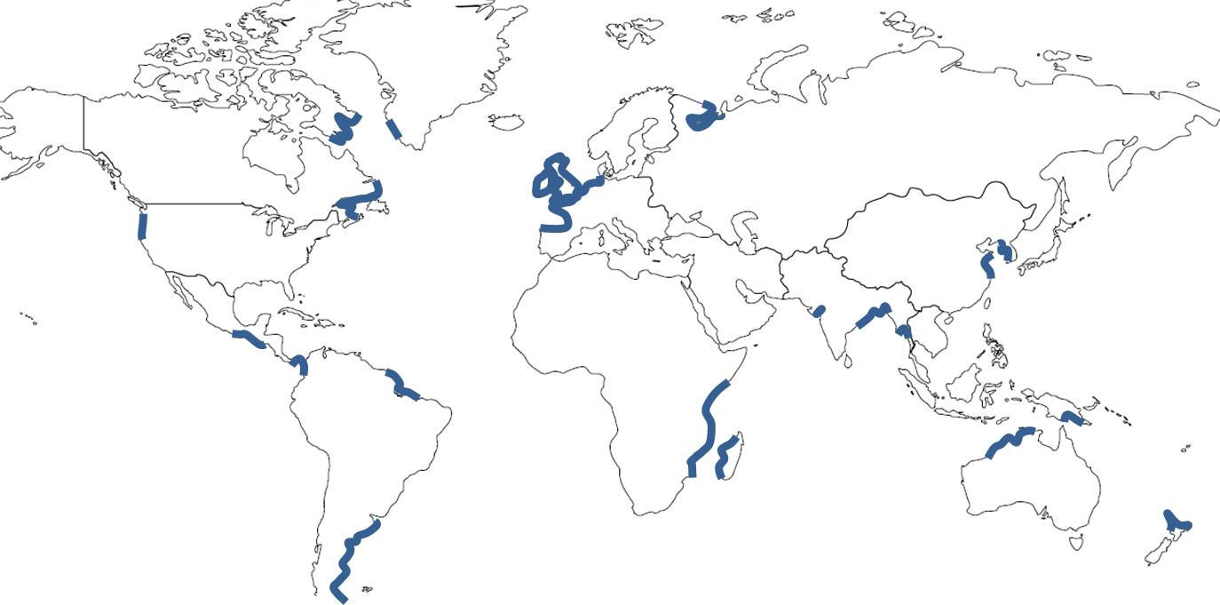
| 16:03, 6 July 2016 | WorldMacroTidalZones.jpg (file) |  |
71 KB | World map of macrotidal coastal zones | 1 |
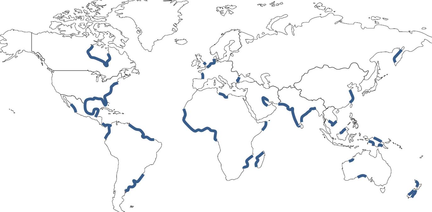
| 16:02, 6 July 2016 | WorldCoastalPlains.jpeg (file) |  |
73 KB | World map of coastal plains | 1 |
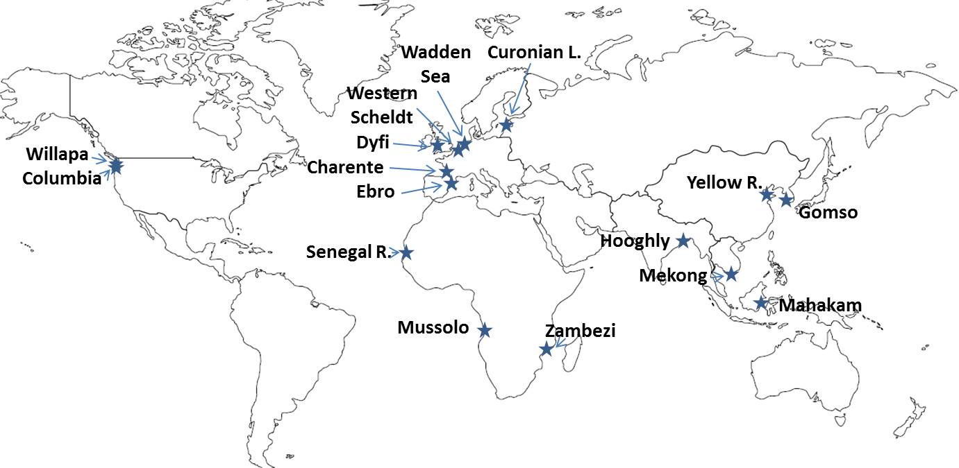
| 16:02, 6 July 2016 | EstuaryLocation.jpeg (file) |  |
88 KB | Location of estuaries discussed in the text on the world map | 1 |
| 16:00, 6 July 2016 | Curonian.jpeg (file) |  |
111 KB | Curonian Lagoon | 1 |
| 15:59, 6 July 2016 | Hooghly.jpeg (file) |  |
113 KB | Hooghly estuary | 1 |
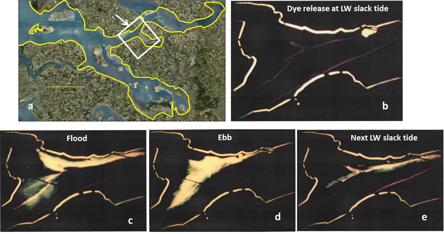
| 10:21, 24 May 2016 | DyeExperiment3.jpg (file) |  |
137 KB | Dye experiment 3. Panel a: Location viewed by the camera. Panels b, c, d, e: dye patch at different tidal phases. | 2 |
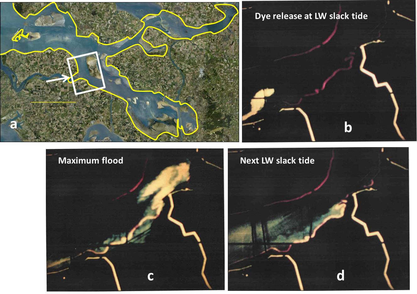
| 10:20, 24 May 2016 | DyeExperiment2.jpg (file) |  |
145 KB | Dye experiment 2. Panel a: Location viewed by the camera. Panels b, c, d: dye patch at different tidal phases. | 2 |