Interpolation of measured grain-size fractions
Contents
Introduction
In marine-habitat and in marine-landscape mapping, information on various physical/abiotic parameters of the area under consideration is important. Along with information on biotic parameters, physical/abiotic parameters are used to define and map habitats or landscapes. One of the most relevant physical parameters used in seabed mapping is the grain size of the sediment. Until now, the most commonly used grain-size descriptor has been the sand median, also known as the Ds50. The median diameter of the sand fraction (defined as the fraction between 63 micron and 2 mm), is the midpoint of the grain-size distribution: 50% (by weight) of the sediment is coarser and 50% is finer than the median grain size. Traditionally, the sand median known from measured points is used to create a full-coverage map by interpolating the measured values. The median is the most widely known grain-size descriptor, because it is easily measured or estimated. However, the sand median is not always the most relevant grain-size descriptor of natural sediment, which usually does not have a log-normal distribution. Bi-modal glacial sediment, for example, cannot be described adequately with only one descriptor. Furthermore, it is statistically not correct to interpolate sand medians, because the sand median is a non-linear parameter and therefore cannot be interpolated linearly. This has been demonstrated in for example Gruijters et al., 2005 [1]. Because of these shortcomings, we took a different approach to come to a more reliable set of grain-size maps. After creating a granulometry database with uniform size-class intervals, we interpolated the measured share of each (cumulative) grain-size fraction for all measured samples.
Location and site details
Thus far, this technique has been applied to data from the entire Dutch Continental Shelf (DCS).
Goals of the mapping
We apply this methodology a) to tackle problems associated with interpolation of sand-median values, and b) to come to more flexible grain-size maps and grids, so that not only the sand median can be extracted but also the D10, D90, or Dx, depending on which descriptor best explains the variation in the biotic data.
Technical outline
As input data, full measured grain-size distributions are used. For the DCS there are 6038 measurements available (December 2006); in the near future, several hundred more measurements will become available, primarily from the northern half of the DCS where coverage is poor at the moment. Main problems with the current set of measurements are:
- Not all grain-size distributions are complete. The fraction >2 mm (the gravel fraction, including shells and shell fragments) is often missing because protocols are not always followed when pre-processing samples for analysis.
- Accurate measurement of mud (silt and clay) content is difficult because of particle agregation during sample processing and because of flocculation under natural conditions. Measured mud percentages are at best a good estimate.
- Sample collection spans a long period, during which various analytical instruments and techniques have been used to measure grain size: several generations of laser-particle sizers (wet and dry), sieving (wet and dry), and the pipette method.
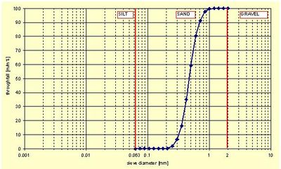
Because of these shortcomings in the data, we focus on the sand fraction only. However, both the very fine (mud) and the coarse fraction (gravel) are important in describing the physical environment, a first approximation is made to include these fractions. Results for the mud fraction are available as a full coverage map, taking the percentage of all particles <63 micron to be a reliable indication of the mud percentage; the gravel fraction will be included as soon as possible. Theses three components, gravel, sand and mud, will be used to make an improved Folk sediment map. During data processing, the class intervals are made uniform, meaning that all measured grain-size distributions are transformed to fit the following 20 fractions: 63-75, 75-88, 88-105, 105-125, 125-150, 150-177, 177-210, 210-250, 250-300, 300-354, 354-420, 420-500, 500-600, 600-707, 707-850, 850-1000, 1000-1190, 1190-1410, 1410-1680, and 1680-2000 micron, conform laser-diffraction fractions used standard within TNO. Taken together, these fractions add up to 100%. For all samples, cumulative grain-size distributions are made (Figure 1).
Figure 1 Example of a cumulative grain-size distribution of the sand fraction.
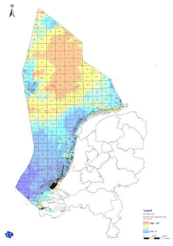
In these graphs the different amounts of throughfall are shown. With a mesh size of 2 mm, 100% of the sediment is falling through. The opposite holds true for a mesh size of 63 micron; 0% of the sediment falls through. These cumulative grain-size distributions are used in interpolation. For that purpose they are exported to geostatistical interpolation software. All fractions are interpolated with a technique called Kriging with External Drift. Verfaillie et al. (2006)[2] describe this technique in detail. Verfaillie et al. illustrate that the bathymetry explains most variation in the sand median. We therefore assume that this is also valid for the separate fractions on which the sand median is based, and use this parameter as external-drift variable. Resulting from this interpolation are full-coverage grids for all fractions. In Figure 2 an example of one of these full-coverage maps can be seen. These grids have to be post processed in order to calculate for example D50, D10 or D90.
Figure 2 Example of full-coverage map of an interpolated fraction, in this case 210 micron.
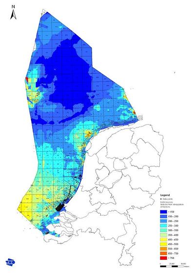
The post processing again consists of several steps. Owing to the interpolation technique used (Kriging), values for throughfall can become more than 100% or less than 0%, when data density is not sufficient. We have to correct for these artificial results, therefore values less than 0% are corrected to 0% and values over 100% are corrected to 100%. Furthermore, we build in a check to force the interpolated values to exactly follow a cumulative grain-size distribution, meaning that on any location, throughfall for a particular mesh size should be less than for a coarser mesh size. Further data post processing is performed with a script in Python. We can calculate whichever D is needed, for example the D10 or D50. The outcome of these calculations can be plotted in any GIS program and can be used afterward in for example marine-landscape mapping or habitat mapping by combining physical and biotic data. In Figure 3 the D50 map for the DCS is showed, calculated with the above explained technique. Clearly recognizable are the large-scale bathymetric features on this map. Also clearly visible is the effect of insufficient data density, which can be seen in the northern part of the DCS. The level of confidence in this area is logically not as high as in areas with sufficient data density.
Figure 3 Ds50 map derived after post-processing of interpolation results for all fractions.
Summary of results
Main results from this study are tailor-made full-coverage sediment maps that are both more accurate and more relevant than existing ones. By using the technique of interpolating grain-size fractions, any D can be calculated, which makes this technique much more flexible than the traditional interpolation of measured D50 values.
Key lessons
Quality of the data used is very important, and so is data density; without a sufficient data density the reliability of the resulting map is uncertain (and most likely limited). One should always keep in mind what kind of natural processes and parameters resulted in the sediment distribution as present in situ. The spatial scales of these processes and parameters should be larger than the distance between data points in order for data points to be correlated. More information on geostatistics is presented by Isaaks et al. (1989)[3].
Conclusions
The technique presented here is a very flexible tool for the construction of full-coverage sediment maps, and can be applied easily when sufficient grain-size data are available in a uniform format.
References
- ↑ Gruijters, S.H.L.L., Maljers, D., Veldkamp, J.G. (2005). 3D interpolation of grain size distributions in the upper 5 m of the channel bed of three lower Rhine distributaries. Physics and Chemistry of the Earth 30: 303-316.
- ↑ Verfaillie, E., Lancker, V. van, Meirvenne, M. van (2006). Multivariate geostatistics for the predictive modelling of the surficial sand distribution in shelf seas. Continental Shelf Research. Volume 26. Issue 19: 2454-2468.
- ↑ Isaaks, E.H., Srivastava, R.M. (1989). An introduction to applied geostatistics. Oxford University Press.
See also
- Coastal and marine sediments
- Data interpolation with Kriging
- Computation of sediment transport and presentation of results
Please note that others may also have edited the contents of this article.
|


