Linear regression analysis of coastal processes
Linear regression analysis of beach level data is demonstrated here using a set of beach profile measurements carried out at locations along the Lincolnshire coast (UK) by the National Rivers Authority (now the Environment Agency) and its predecessors between 1959 and 1991, as described in Sutherland et al. 2007[1]. A short introduction to linear regression theory is given in Appendix A.
Contents
Use of trend line for prediction
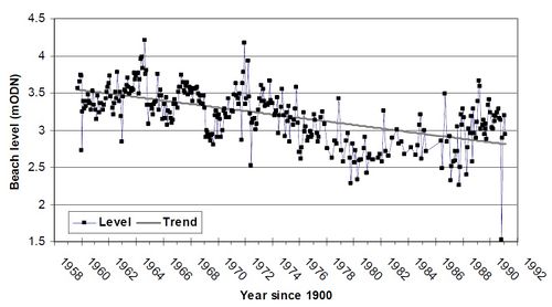
In order to better understand and predict beach level lowering in front of a seawall, beach levels were measured in front of seawalls along the Lincolnshire coast (UK). Figure 1 shows the bed level change measured in front of the seawall at Mablethorpe Convalescent Home.
Straight lines fitted to beach level time series give an indication of the rate of change of elevation and hence of erosion or accretion. The measured rates of change are often used to predict future beach levels by assuming that the best-fit rate from one period will be continued into the future. Alternatively, long-term shoreline change rates can be determined using linear regression on cross-shore position versus time data.
Genz et al. (2007)[2] reviewed methods of fitting trend lines, including using end point rates, the average of rates, ordinary least squares (including variations such as jackknifing, weighted least squares and least absolute deviation (with and without weighting functions). Genz et al. recommended that weighted methods should be used if uncertainties are understood, but not otherwise. The ordinary least squares, jackknifing and least absolute deviation methods were preferred (with weighting, if appropriate). If the uncertainties are unknown or not quantified then the least absolute deviation methods is preferred.

The following question then arises: how useful is a best-fit linear trend as a predictor of future beach levels? In order to examine this, the thirty years of Lincolnshire data have been divided into sections: from 1960 to 1970, from 1970 to 1980, from 1980 to 1990 and from 1960 to 1990, for most of the stations. In each case a least-squares best-fit straight line was fitted to the data and the rates of change in elevation from the different periods are shown below:
- From 1960 to 1970 the rate of change was -17mm/year;
- From 1970 to 1980 the rate of change was -63mm/year;
- From 1980 to 1990 the rate of change was +47mm/year.
- From 1960 to 1990 the rate of change was -25mm/year.
The data above indicates that 10-year averages provide little predictive capability for estimating the change in elevation for the next 10-years, let alone for the planning horizon that might need to be considered for a coastal engineering scheme. Few of the 10-year averages are close to the 30-year average.
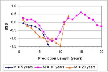
A prediction horizon is defined as the average length of time over which a prediction (here an extrapolated trend) produces a better level of prediction of future beach levels than a simple baseline prediction. Sutherland et al. (2007)[1] devised a method of determining the prediction horizon for an extrapolated trend using the Brier Skill Score (Sutherland et al., 2004[3]). Here the baseline prediction was that future beach levels would be the same as the average of the measured levels used to define the trend. A 10 year trend was found to have a prediction horizon of 4 years at Mablethorpe Convalescent Home (Fig. 2). Similar values have been found at other sites in Lincolnshire.
For a discussion of beach lowering in front of seawalls see also the article Seawalls and revetments.
Conditions for application
Assumptions underlying regression analysis and least-square fitting are:
- the deviations from the trend curve can be equated with Gauss-distributed random noise;
- the deviations are uncorrelated.
In the example of Mablethorpe beach the distribution of residual (i.e. de-trended) beach levels seems to follow the common assumption of a Gaussian (normal) distribution, as shown in Fig. 3.
If the data have random fluctuations which are significantly correlated over some distance, other regression methods must be used. Frequently used analysis methods in this case are:
Appendix A: Introduction to linear regression theory
Although regression analysis is explained in many textbooks, a short mathematical introduction is given below. The object of linear regression is to analyze the correlation of a measurable property [math]h[/math] (the so-called 'dependent variable' or 'target') with a number [math]K-1[/math] measurable factors [math]y_k, \; k=2, .., K[/math] (the 'independent variables' or 'regressors'). Linear regression is based on the assumption that [math]h[/math] can be estimated through a linear relationship:
[math]h = \hat{h} +\epsilon \; , \quad \hat{h} = a_1 + \sum_{k=2}^K a_k y_k = \sum_{k=1}^K a_k y_k \; , \qquad (A1)[/math]
where [math]\hat{h}[/math] is the estimator, [math]a_k, \; k=2, .., K[/math] are the regression coefficients, [math]a_1[/math] is the intercept and [math]y_1=1[/math]. The term [math]\epsilon[/math] is the 'error', i.e., the difference between the true value [math]h[/math] and the estimator [math]\hat{h}[/math]. (Note: Linear regression means linear in the regression coefficients; the regressors [math]y_k[/math] can be nonlinear quantities, for example [math]y_3=y_2^2[/math].) Now assume that we have observations of [math]N[/math] different instances of the [math]K-1[/math] regressors, [math]y_{ki}, \; i=1, .., N[/math], and corresponding observations of the dependent variable, [math]h_i[/math]. If [math]N\gt K[/math] these observations can be used to estimate the values of the regression coefficients [math]a_k[/math] by looking for the best solution to the linear system
[math]h_i = \sum_{k=1}^K a_k y_{ki} + \epsilon_i \; , \qquad (A2)[/math]
where [math]\epsilon_i[/math] are errors related to: (i) the approximate validity of the linear estimator (sometimes called 'epistemic uncertainty') and (ii) measurement inaccuracies, which are often statistical ('aleatoric') uncertainties. The errors are considered to be stochastic variables with zero mean, [math]E[\epsilon_i]=0[/math] and variance [math]\sigma_i^2 \equiv E[\epsilon_i^2][/math] (we use the notation [math]E[x][/math]= the mean value from a large number of trials of the stochastic variable [math]x[/math]).
What is 'the best solution"? Different criteria can be used. Least square optimization is the most often used criterium, i.e., the solution for which the sum of the squared errors [math]\Phi[/math] is minimum,
[math]\Phi = ½ \sum_{i=1}^N \epsilon_i^2 = ½ \sum_{i=1}^N \sum_{j=1}^N \big(h_i - \sum_{k=1}^K a_k y_{ki}\big) \big(h_j - \sum_{k'=1}^K a_{k'} y_{k'j}\big) . \qquad (A3)[/math]
At minimum, [math]\Phi[/math] increases for any change in one of the coefficients [math]a_k[/math], which implies that the partial derivatives are zero:
[math]\Large\frac{\partial \Phi}{\partial a_k}\normalsize = 0 , \; k=1, ..,K . \qquad (A4)[/math]
This condition yields the set of [math]K[/math] linear equations
[math] - \sum_{i=1}^N y_{ki} h_i + \sum_{i=1}^N \sum_{k'=1}^K y_{ki} y_{k'i} a_{k'} = 0 . \qquad (A5)[/math]
from which the regression coefficients [math]a_k[/math] can be solved.
In the more compact matrix notation we may write: [math]H[/math] is the [math]N[/math]-vector with elements [math]h_i[/math], [math]\; A[/math] is the [math]K[/math]-vector with elements [math]a_k[/math] and [math]Y[/math] is the [math]K \times N[/math] matrix with elements [math]y_{ki}[/math]. The linear equations (A5) can then be written
[math]Y^T \, H = Y^T \, Y \, A . \qquad (A6)[/math]
The solution is found by inversion of the [math]N \times N[/math] matrix [math]Y^T \, Y[/math], giving
[math]A = (Y^T \, Y)^{-1} Y^T \, H . \qquad (A7)[/math]
Least squares is the best solution if the regressors [math]y_k[/math] are uncorrelated and if the errors [math]\epsilon_i[/math] are uncorrelated and identically Gaussian-distributed, i.e., they all have the same variance [math]\sigma_i^2[/math]. This is often not the case in practice. A few other cases are discussed below.
Case 1. The data have errors that scale with their magnitude. Then a log transform of the data produces errors approximately independent of the magnitude. Linear regression with least squares is applied to the log-transformed data.
Case 2. The errors differ among the data ('non-homoscedasticity'), [math]\sigma_i \ne \sigma_j , \, i \ne j[/math]. If estimates of the variances are known, one can use weighted least squares instead of least squares, i.e., replace (A3) with [math]\Phi = ½ \sum_{i=1}^N \big( \epsilon_i / \sigma_i \big)^2[/math].
Case 3. Multicollinearity, meaning a linear relationship exists between two or more regressor variables. In this case the non-independent regressor variable should be removed from the data.
Case 4. The errors of the [math]N[/math] observations are correlated, [math]c_{ij} \equiv E[\epsilon_i \, \epsilon_j] \ne 0[/math]. If an estimate of the covariances [math]c_{ij} [/math] is known, the generalized least squares method can be used. The solution (A7) is then replaced by
[math]A = (Y^T \, C^{-1} \, Y)^{-1} Y^T \, C^{-1} H , \qquad (A8)[/math]
where [math]C[/math] is the covariance matrix with elements [math]c_{ij}[/math]. Another option is to use kriging, see the article Data interpolation with Kriging.
Related articles
References
- ↑ 1.0 1.1 1.2 Sutherland, J., Brampton, A.H., Obhrai, C., Motyka, G.M., Vun, P.-L. and Dunn, S.L. 2007. Understanding the lowering of beaches in front of coastal defence structures, Stage 2. Defra/EA Joint Flood and Coastal Erosion Risk Management R&D programme Technical Report FD1927/TR
- ↑ Genz, A.S., Fletcher, C.H., Dunn, R.A., Frazer, L.N. and Rooney, J.J. 2007. The predictive accuracy of shoreline change rate methods and alongshore beach variation on Maui, Hawaii. Journal of Coastal Research 23(1): 87 – 105
- ↑ Sutherland, J., Peet, A.H. and Soulsby, R.L. 2004. Evaluating the performance of morphological models. Coastal Engineering 51, pp. 917-939.
Please note that others may also have edited the contents of this article.
|

