Using model simulations to support monitoring - Implementation & Results
Contents
Introduction
The examples discussed below summarise the use of model simulations in the context of different monitoring programmes. Only one example, the interpretation of FerryBox observations, does not explicitly emphasise the long-term aspect of monitoring. Instead it takes advantage of the fact that model simulations stored in coastDat provide detailed reconstructions of environmental conditions rather than just statistics of natural variability. The same kind of detailed information is exploited in the project on survey data of oil contaminated beached birds. In the latter case, however, the analysis is performed on another level of temporal aggregation being set by the schedule of the fortnightly observations. In the analysis of freshwater signals observed at Helgoland the relevant time scale is somewhat in between.
Fresh water signals at Helgoland
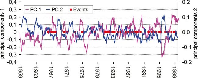
In 1962 a long-term pelagic monitoring programme, including plankton species composition, was startet at the island of Helgoland (Helgoland Roads, 54°11.3’N, 7°54.0’E) in the North Sea by the Biologische Anstalt Helgoland on a work-daily basis (Franke et al., 2004[1] ). An important aspect for the interpretation of the long term data is the distinction between substantial changes within the biological network and changes that reflect variations or trends of the hydrodynamic regime. The coastDat data starting at 1958 covers the whole period of the Helgoland Roads observations and thus allows to demonstrate the added value which can be gained from combining long term biological observations with model based hindcasts of physical environmental conditions. Hydrodynamic changes on various time scales must be taken into account for a meaningful interpretation of *biological time series. Fig. 1 demonstrates the general idea by a simple example dealing with the interpretation of changes in the frequency of freshwater signals that have been observed at Helgoland Roads during the last decades. According to Fig. 1 these changes are consistent with a simulated changing variability of the dominant flow patterns in the German Bight.
Oil contaminated beached birds
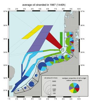
Chronic oil pollution in the German Bight resulting from illegal oil dumping by ships is a severe problem that harms the marine environment. It is difficult to quantify, although model based estimates are possible (Fig. 2). The number of oil-contaminated beached birds is often used as an indicator for trends in the level of chronic oil pollution. It turns out,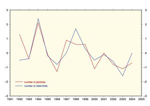
however, that data from such surveys may easily be misinterpreted if the variability of wind conditions is not properly taken into account. Fig. 3 shows that within a period of 13 years, for which reliable observations exist, changing atmospheric winter conditions might lead us to believe in a decreasing trend of oil pollution. The example clearly shows that a careful analysis of environmental conditions is indispensable for a sound and reliable interpretation of the results of the beached birds monitoring programme.
FerryBox and station Gabbard
Modelling of marine circulation offers several options for taking maximum advantage of observations that are made on moving platforms. Hydrodynamic drift modelling can be used to establish a link with observations from any other station. It can also be used for the construction of synoptic spatial distributions from non-synoptic observations along a given transect.
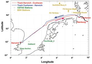
The example given here deals with the comparison of FerryBox salinity observations and corresponding observations at Gabbard station. Even though the ferry route passes close to Gabbard station (Fig. 4), a direct comparison of the respective observations is not successful due to small scale variability in the area of interest. According to Fig. 5, however, using the drift model as a link, the comparison can be much improved. A more detailed analysis of the method’s performance reveals problems in those cases when FerryBox observations are taken close to the English coast. The reason for this failure may be either small scale patchiness of salinity or insufficient model resolution inshore.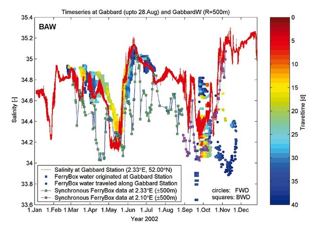
Related articles
- Coastal observation systems
- FerryBox - Continuous and automatic water quality observations along transects
- Ships of opportunity and ferries as instrument carriers
References
- ↑ Franke, H.-D., Buchholz, F. & Wiltshire, K.H. (2004). Ecological long-term research at Helgoland (German Bight, North Sea): retrospect and prospect – an introduction. Helgoland Marine Research, 58, 223-229.
Please note that others may also have edited the contents of this article.
|
Please note that others may also have edited the contents of this article.
|
Please note that others may also have edited the contents of this article.
|
Please note that others may also have edited the contents of this article.
|
Please note that others may also have edited the contents of this article.
|
Please note that others may also have edited the contents of this article.
|
